ggalluvial/ 0000755 0001762 0000144 00000000000 15146573312 012410 5 ustar ligges users ggalluvial/tests/ 0000755 0001762 0000144 00000000000 15146567322 013556 5 ustar ligges users ggalluvial/tests/testthat/ 0000755 0001762 0000144 00000000000 15146573312 015412 5 ustar ligges users ggalluvial/tests/testthat/test-stat-stratum.r 0000644 0001762 0000144 00000004363 14452602415 021224 0 ustar ligges users # weights are used but not returned
test_that("`stat_stratum` weights computed variables but drops weight", {
data <- data.frame(x = rep(1:2, c(2, 3)), stratum = LETTERS[c(1, 2, 1, 2, 2)])
data$y <- c(1, 1, 1, 1, 2)
data$weight <- c(.5, 1, .5, 1, 1.5)
comp <- StatStratum$compute_panel(data)
comp <- comp[with(comp, order(x, stratum)), ]
expect_equivalent(comp$n, c(0.5, 1, 0.5, 2.5))
expect_equivalent(comp$count, c(0.5, 1, 0.5, 4))
expect_equivalent(comp$prop, c(c(1, 2) / 3, c(1, 8) / 9))
expect_null(comp$lode)
expect_null(comp$weight)
})
# reverse and absolute parameters, negative values
test_that("`stat_stratum` orders strata correctly with negative values", {
data <- expand.grid(stratum = LETTERS[1:2], x = 1:2)
data$y <- c(1, 1, -1, -1)
# order by stratum, `reverse = TRUE`
#ggplot(data, aes(x = x, stratum = stratum, y = y)) +
# geom_stratum() +
# geom_text(stat = "stratum", aes(label = stratum))
comp <- StatStratum$compute_panel(data)
expect_identical(comp[with(comp, order(x, stratum)), ]$y,
c(1.5, 0.5, -1.5, -0.5))
# order by stratum, `reverse = FALSE`
#ggplot(data, aes(x = x, stratum = stratum, y = y)) +
# geom_stratum(reverse = FALSE) +
# geom_text(stat = "stratum", aes(label = stratum), reverse = FALSE)
comp <- StatStratum$compute_panel(data, reverse = FALSE)
expect_identical(comp[with(comp, order(x, stratum)), ]$y,
c(0.5, 1.5, -0.5, -1.5))
# order by stratum, `absolute = FALSE`
#ggplot(data, aes(x = x, stratum = stratum, y = y)) +
# geom_stratum(absolute = FALSE) +
# geom_text(stat = "stratum", aes(label = stratum), absolute = FALSE)
comp <- StatStratum$compute_panel(data, absolute = FALSE)
expect_identical(comp[with(comp, order(x, stratum)), ]$y,
c(1.5, 0.5, -0.5, -1.5))
# order by stratum, `reverse = FALSE, absolute = FALSE`
#ggplot(data, aes(x = x, stratum = stratum, y = y)) +
# geom_stratum(reverse = FALSE, absolute = FALSE) +
# geom_text(stat = "stratum", aes(label = stratum),
# reverse = FALSE, absolute = FALSE)
comp <- StatStratum$compute_panel(data, reverse = FALSE, absolute = FALSE)
expect_identical(comp[with(comp, order(x, stratum)), ]$y,
c(0.5, 1.5, -1.5, -0.5))
})
ggalluvial/tests/testthat/test-geom-stratum.r 0000644 0001762 0000144 00000002255 14452602415 021176 0 ustar ligges users # visual tests
test_that("`geom_stratum` draws correctly", {
d <- as.data.frame(Titanic)
a1 <- aes(y = Freq, axis1 = Class, axis2 = Sex, axis3 = Age, axis4 = Survived)
a2 <- aes(y = Freq, axis1 = Class, axis2 = Sex)
skip_on_cran()
skip_if_not_installed("vdiffr")
vdiffr::expect_doppelganger(
"`geom_stratum`: basic",
ggplot(d, a1) + geom_stratum()
)
vdiffr::expect_doppelganger(
"`geom_stratum`: extended width",
ggplot(d, a1) + geom_stratum(width = 1)
)
vdiffr::expect_doppelganger(
"`geom_stratum`: inferred text labels",
ggplot(d, a1) +
geom_text(stat = "stratum", aes(label = after_stat(stratum)))
)
vdiffr::expect_doppelganger(
"`geom_stratum`: axis labels",
ggplot(d, a1) + geom_stratum() +
scale_x_discrete(limits = c("Class", "Sex", "Age", "Survived"))
)
vdiffr::expect_doppelganger(
"`geom_stratum`: facets",
ggplot(d, a2) + geom_stratum() +
facet_wrap(~ Age, scales = "free_y")
)
vdiffr::expect_doppelganger(
"`geom_stratum`: facets and axis labels",
ggplot(d, a2) + geom_stratum() +
scale_x_discrete(limits = c("Class", "Sex")) +
facet_wrap(~ Age, scales = "free_y")
)
})
ggalluvial/tests/testthat/test-geom-alluvium.r 0000644 0001762 0000144 00000007220 14704334714 021336 0 ustar ligges users # visual tests
test_that("`geom_alluvium` draws correctly", {
skip_on_cran()
skip_if_not_installed("vdiffr")
d1 <- as.data.frame(Titanic)
a1 <- aes(y = Freq, axis1 = Class, axis2 = Sex, axis3 = Age, fill = Survived)
a2 <- aes(y = Freq, axis1 = Class, axis2 = Sex)
vdiffr::expect_doppelganger(
"`geom_alluvium`: basic",
ggplot(d1, a1) + geom_alluvium()
)
vdiffr::expect_doppelganger(
"`geom_alluvium`: facets",
ggplot(d1, a2) +
geom_alluvium(aes(fill = Age), width = .4) +
facet_wrap(~ Survived, scales = "fixed")
)
skip_if_not_installed("alluvial")
d2 <- alluvial::Refugees
a3 <- aes(y = refugees, x = year, alluvium = country)
vdiffr::expect_doppelganger(
"`geom_alluvium`: bump plot",
ggplot(d2, a3) +
geom_alluvium(aes(fill = country), width = 1/4, decreasing = FALSE)
)
vdiffr::expect_doppelganger(
"`geom_alluvium`: line plot",
ggplot(d2, a3) +
geom_alluvium(aes(fill = country),
width = 0, knot.pos = 0, outline.type = "upper")
)
})
test_that("`geom_alluvium()` recognizes alternative curves", {
data(vaccinations)
skip_on_cran()
skip_if_not_installed("vdiffr")
suppressWarnings(vdiffr::expect_doppelganger(
"`geom_alluvium`: unscaled knot positions",
ggplot(vaccinations,
aes(x = survey, stratum = response, alluvium = subject,
y = freq, fill = response)) +
geom_alluvium(knot.prop = FALSE)
))
suppressWarnings(vdiffr::expect_doppelganger(
"`geom_alluvium`: 'linear' curve",
ggplot(vaccinations,
aes(x = survey, stratum = response, alluvium = subject,
y = freq, fill = response)) +
geom_alluvium(curve_type = "linear")
))
suppressWarnings(vdiffr::expect_doppelganger(
"`geom_alluvium`: 'cubic' curve",
ggplot(vaccinations,
aes(x = survey, stratum = response, alluvium = subject,
y = freq, fill = response)) +
geom_alluvium(curve_type = "cubic")
))
suppressWarnings(vdiffr::expect_doppelganger(
"`geom_alluvium`: 'quintic' curve",
ggplot(vaccinations,
aes(x = survey, stratum = response, alluvium = subject,
y = freq, fill = response)) +
geom_alluvium(curve_type = "quintic")
))
suppressWarnings(vdiffr::expect_doppelganger(
"`geom_alluvium`: 'sine' curve",
ggplot(vaccinations,
aes(x = survey, stratum = response, alluvium = subject,
y = freq, fill = response)) +
geom_alluvium(curve_type = "sine")
))
suppressWarnings(vdiffr::expect_doppelganger(
"`geom_alluvium`: 'arctangent' curve",
ggplot(vaccinations,
aes(x = survey, stratum = response, alluvium = subject,
y = freq, fill = response)) +
geom_alluvium(curve_type = "arctan")
))
suppressWarnings(vdiffr::expect_doppelganger(
"`geom_alluvium`: 'arctangent' curve with custom range",
ggplot(vaccinations,
aes(x = survey, stratum = response, alluvium = subject,
y = freq, fill = response)) +
geom_alluvium(curve_type = "arctan", curve_range = 1)
))
suppressWarnings(vdiffr::expect_doppelganger(
"`geom_alluvium`: 'sigmoid' curve",
ggplot(vaccinations,
aes(x = survey, stratum = response, alluvium = subject,
y = freq, fill = response)) +
geom_alluvium(curve_type = "sigmoid")
))
suppressWarnings(vdiffr::expect_doppelganger(
"`geom_alluvium`: 'sigmoid' curve with custom range",
ggplot(vaccinations,
aes(x = survey, stratum = response, alluvium = subject,
y = freq, fill = response)) +
geom_alluvium(curve_type = "sigmoid", curve_range = 3)
))
})
ggalluvial/tests/testthat/test-stat-flow.r 0000644 0001762 0000144 00000007504 14452602415 020474 0 ustar ligges users # weights are used but not returned
test_that("`stat_flow` weights computed variables but drops weight", {
data <- expand.grid(alluvium = letters[1:3], x = 1:2)
data$stratum <- LETTERS[c(1, 1, 2, 1, 2, 2)]
data$y <- c(1, 1, 1, 1, 1, 2)
data$weight <- c(.5, 1, 1, .5, 1, 1)
comp <- as.data.frame(StatFlow$compute_panel(data))
comp <- comp[with(comp, order(x, alluvium)), ]
expect_equivalent(comp$n, c(1, 1, 0.5, 1, 1, 0.5))
expect_equivalent(comp$count, c(1, 1, 0.5, 2, 1, 0.5))
expect_equivalent(comp$prop, c(c(2, 2, 1) / 5, c(4, 2, 1) / 7))
expect_equal(comp$lode, rep(factor(letters[3:1]), times = 2))
expect_null(comp$weight)
})
# reverse and absolute, negative values
test_that("`stat_flow` orders flows correctly with negative values", {
data <- expand.grid(alluvium = letters[1:3], x = 1:2)
data$stratum <- LETTERS[c(1, 1, 2)]
data$y <- c(1, 1, 1, -1, 1, -1)
# order by stratum, `reverse = TRUE`
#ggplot(data, aes(x = x, stratum = stratum, alluvium = alluvium, y = y)) +
# geom_flow()
comp <- StatFlow$compute_panel(data)
expect_identical(comp[with(comp, order(x, alluvium)), ]$y,
c(1.5, 0.5, 2.5, -1.5, -0.5, 0.5))
# order by stratum, `reverse = FALSE`
#ggplot(data, aes(x = x, stratum = stratum, alluvium = alluvium, y = y)) +
# geom_flow(reverse = FALSE)
comp <- StatFlow$compute_panel(data, reverse = FALSE)
expect_identical(comp[with(comp, order(x, alluvium)), ]$y,
c(2.5, 0.5, 1.5, -1.5, -0.5, 0.5))
# order by stratum, `reverse = FALSE, absolute = FALSE`
#ggplot(data, aes(x = x, stratum = stratum, alluvium = alluvium, y = y)) +
# geom_flow(reverse = FALSE, absolute = FALSE)
comp <- StatFlow$compute_panel(data, reverse = FALSE, absolute = FALSE)
expect_identical(comp[with(comp, order(x, alluvium)), ]$y,
c(0.5, 2.5, 1.5, -1.5, -0.5, 0.5))
})
# aesthetic binding
test_that("`stat_flow` orders alluvia correctly according to `aes.bind`", {
data <- expand.grid(alluvium = letters[1:4], x = 1:2)
data$stratum <- LETTERS[c(1, 1, 1, 2, 2, 1, 3, 1)]
data$y <- 1
data$fill <- c("red", "blue", "blue", "blue",
"red", "blue", "blue", "blue")
# order by index strata and linked strata (flows)
#ggplot(data, aes(x = x, stratum = stratum, alluvium = alluvium, y = y)) +
# geom_flow(aes(fill = fill))
comp <- StatFlow$compute_panel(data)
expect_identical(comp[with(comp, order(x, alluvium)), ]$y,
c(2.5, 1.5, 0.5, 3.5, 1.5, 0.5, 2.5, 3.5))
# order by index strata, linked strata (flows), and aesthetics
#ggplot(data, aes(x = x, stratum = stratum, alluvium = alluvium, y = y)) +
# geom_flow(aes(fill = fill), aes.bind = "flows")
comp <- StatFlow$compute_panel(data, aes.bind = "flows")
expect_identical(comp[with(comp, order(x, alluvium)), ]$y,
c(1.5, 2.5, 0.5, 3.5, 1.5, 0.5, 2.5, 3.5))
# cannot order by aesthetics before by linked strata (flows)
expect_warning(StatFlow$compute_panel(data, aes.bind = "alluvia"), "flows")
})
# missing values
test_that("`stat_flow` preserves missingness to position flows", {
data <- data.frame(x = c(1, 2, 2, 3),
stratum = factor(LETTERS[c(1L, 2L, 1L, 2L)]),
alluvium = c(1L, 2L, 1L, 2L),
PANEL = factor(1L),
group = seq(4L),
y = 1)
comp <- StatFlow$compute_panel(data)
expect_identical(sort(complete.cases(comp)), rep(c(FALSE, TRUE), c(2L, 4L)))
})
# exceptional data
test_that("`stat_flow` handles exceptional data with out errors", {
wph <- as.data.frame(as.table(WorldPhones))
names(wph) <- c("Year", "Region", "Telephones")
wph$Year <- as.integer(as.character(wph$Year))
gg <- ggplot(wph, aes(x = Year, alluvium = Region, y = Telephones)) +
geom_flow(aes(fill = Region, colour = Region))
expect_silent(ggplot_build(gg))
})
ggalluvial/tests/testthat/test-alluvial-data.r 0000644 0001762 0000144 00000007327 14452602415 021277 0 ustar ligges users titanic_alluvia <- as.data.frame(Titanic)
null_wt <- NULL
# `is_alluvia_form()` tests
test_that("`is_alluvia_form` recognizes alluvia-format Titanic data", {
expect_message(is_alluvia_form(titanic_alluvia), "[Mm]issing")
expect_true(is_alluvia_form(titanic_alluvia, axes = c("Class", "Sex")))
expect_true(is_alluvia_form(titanic_alluvia, axes = 1:4))
expect_true(is_alluvia_form(titanic_alluvia, Class, Sex, Age))
expect_true(is_alluvia_form(titanic_alluvia, axes = c("Class", "Sex"),
weight = "Freq"))
expect_true(is_alluvia_form(titanic_alluvia, axes = 1:4, weight = 5))
expect_true(is_alluvia_form(titanic_alluvia, Class, Sex, Age, weight = Freq))
expect_true(is_alluvia_form(titanic_alluvia, Class, Sex, weight = !!null_wt))
})
# `to_lodes_form()` tests
test_that("`to_lodes_form` consistently formats Titanic data", {
expect_equivalent(to_lodes_form(titanic_alluvia, axes = c("Class", "Sex")),
to_lodes_form(titanic_alluvia, axes = 1:2))
expect_equivalent(to_lodes_form(titanic_alluvia, axes = c("Class", "Sex")),
to_lodes_form(titanic_alluvia, Class, Sex))
expect_equivalent(to_lodes_form(titanic_alluvia, axes = c("Class", "Sex"),
diffuse = "Class"),
to_lodes_form(titanic_alluvia, axes = 1:2,
diffuse = 1))
expect_equivalent(to_lodes_form(titanic_alluvia, axes = c("Class", "Sex"),
diffuse = "Class"),
to_lodes_form(titanic_alluvia, Class, Sex,
diffuse = Class))
})
# preparation for next tests
titanic_lodes <- suppressWarnings(to_lodes_form(
transform(titanic_alluvia, Index = 1:nrow(titanic_alluvia)),
key = "Variable", value = "Value", id = "Index", axes = 1:4,
factor_key = TRUE
))
titanic_lodes$Value <-
factor(titanic_lodes$Value,
levels = do.call(c, lapply(titanic_alluvia[, 1:4], levels)))
# `is_lodes_form()` tests
test_that("`is_lodes_form` recognizes lodes-format Titanic data", {
expect_error(is_lodes_form(titanic_lodes))
expect_true(is_lodes_form(titanic_lodes,
key = "Variable", value = "Value", id = "Index"))
expect_true(is_lodes_form(titanic_lodes,
key = Variable, value = Value, id = Index))
expect_true(is_lodes_form(titanic_lodes,
key = 3, value = 4, id = 2))
expect_true(is_lodes_form(titanic_lodes,
key = "Variable", value = "Value", id = "Index",
weight = "Freq"))
expect_true(is_lodes_form(titanic_lodes,
key = 3, value = 4, id = 2,
weight = 1))
expect_true(is_lodes_form(titanic_lodes,
key = Variable, value = Value, id = Index,
weight = Freq))
expect_true(is_lodes_form(titanic_lodes,
key = Variable, value = Value, id = Index,
weight = !!null_wt))
})
# `to_alluvia_form()` tests
test_that("`to_alluvia_form` consistently formats Titanic data", {
expect_equivalent(to_alluvia_form(titanic_lodes,
key = "Variable", value = "Value",
id = "Index"),
to_alluvia_form(titanic_lodes,
key = 3, value = 4, id = 2))
expect_equivalent(to_alluvia_form(titanic_lodes,
key = "Variable", value = "Value",
id = "Index"),
to_alluvia_form(titanic_lodes,
key = Variable, value = Value, id = Index))
})
ggalluvial/tests/testthat/test-stat-alluvium.r 0000644 0001762 0000144 00000010702 15042736161 021357 0 ustar ligges users # weights are used but not returned
test_that("`stat_alluvium` weights computed variables but drops weight", {
# not cementing alluvia
data <- expand.grid(alluvium = letters[1:3], x = 1:2)
data$stratum <- LETTERS[c(1, 1, 2, 1, 2, 2)]
data$y <- c(1, 1, 1, 1, 1, 2)
data$weight <- c(.5, 1, 1, .5, 1, 1)
comp <- StatAlluvium$compute_panel(data)
comp <- comp[with(comp, order(x, alluvium)), ]
expect_equivalent(comp$n, c(0.5, 1, 1, 0.5, 1, 1))
expect_equivalent(comp$count, c(0.5, 1, 1, 0.5, 1, 2))
expect_equivalent(comp$prop, c(c(1, 2, 2) / 5, c(1, 2, 4) / 7))
expect_equal(comp$lode, factor(rep(letters[1:3], times = 2)))
expect_null(comp$weight)
# cementing alluvia
data$stratum <- LETTERS[c(1, 1, 2)]
comp <- StatAlluvium$compute_panel(data, cement.alluvia = TRUE)
comp <- comp[with(comp, order(x, alluvium)), ]
expect_equivalent(comp$n, c(1.5, 1, 1.5, 1))
expect_equivalent(comp$count, c(1.5, 1, 1.5, 2))
expect_equivalent(comp$prop, c(c(3, 2) / 5, c(3, 4) / 7))
expect_equal(comp$lode, rep(factor(letters[1:3])[c(1, 3)], times = 2))
expect_null(comp$weight)
})
# negative values
test_that("`stat_alluvium` orders alluvia without regard to negative values", {
data <- expand.grid(alluvium = letters[1:2], x = 1:2)
data$stratum <- LETTERS[1]
data$y <- c(-1, -1)
# order by alluvium, `reverse = TRUE`
#ggplot(data, aes(x = x, stratum = stratum, alluvium = alluvium, y = y)) +
# geom_alluvium() +
# geom_text(stat = "alluvium", aes(label = alluvium))
comp <- StatAlluvium$compute_panel(data)
expect_identical(comp[with(comp, order(x, alluvium)), ]$y,
c(-0.5, -1.5, -0.5, -1.5))
# order by alluvium, `reverse = FALSE`
#ggplot(data, aes(x = x, stratum = stratum, alluvium = alluvium, y = y)) +
# geom_alluvium(absolute = FALSE) +
# geom_text(stat = "alluvium", aes(label = alluvium), absolute = FALSE)
comp <- StatAlluvium$compute_panel(data, absolute = FALSE)
expect_identical(comp[with(comp, order(x, alluvium)), ]$y,
c(-0.5, -1.5, -0.5, -1.5))
})
# aesthetic binding
test_that("`stat_alluvium` orders alluvia correctly according to `aes.bind`", {
data <- expand.grid(alluvium = letters[1:4], x = 1:2)
data$stratum <- LETTERS[1:2][c(1, 1, 2, 2, 2, 2, 2, 1)]
data$y <- 1
data$fill <- c("red", "blue", "blue", "blue")
# order by index strata, linked strata (flows), and alluvia
#ggplot(data, aes(x = x, stratum = stratum, alluvium = alluvium, y = y)) +
# geom_alluvium(aes(fill = fill)) +
# geom_text(stat = "alluvium", aes(fill = fill, label = alluvium))
comp <- StatAlluvium$compute_panel(data)
expect_identical(comp[with(comp, order(x, alluvium)), ]$y,
c(3.5, 2.5, 0.5, 1.5, 2.5, 1.5, 0.5, 3.5))
# order by index strata, linked strata (flows), aesthetics, and alluvia
#ggplot(data, aes(x = x, stratum = stratum, alluvium = alluvium, y = y)) +
# geom_alluvium(aes(fill = fill), aes.bind = "flows") +
# geom_text(stat = "alluvium", aes(fill = fill, label = alluvium),
# aes.bind = "flows")
comp <- StatAlluvium$compute_panel(data, aes.bind = "flows")
expect_identical(comp[with(comp, order(x, alluvium)), ]$y,
c(2.5, 3.5, 0.5, 1.5, 1.5, 2.5, 0.5, 3.5))
# order by index strata, aesthetics, linked strata (flows), and alluvia
#ggplot(data, aes(x = x, stratum = stratum, alluvium = alluvium, y = y)) +
# geom_alluvium(aes(fill = fill), aes.bind = "alluvia") +
# geom_text(stat = "alluvium", aes(fill = fill, label = alluvium),
# aes.bind = "alluvia")
comp <- StatAlluvium$compute_panel(data, aes.bind = "alluvia")
expect_identical(comp[with(comp, order(x, alluvium)), ]$y,
c(2.5, 3.5, 0.5, 1.5, 0.5, 2.5, 1.5, 3.5))
})
# exceptional data
test_that("`stat_flow` handles exceptional data with out errors", {
skip_if_not_installed("alluvial")
data(Refugees, package = "alluvial")
refugees_sub <- subset(Refugees, year %in% c(2003, 2005, 2010, 2013))
gg <- ggplot(refugees_sub, aes(x = year, y = refugees, alluvium = country)) +
geom_alluvium(aes(fill = country))
expect_silent(ggplot_build(gg))
})
d <- data.frame(
subject = rep(c("A", "B"), each = 2),
time = rep(1:2, times = 2),
status = factor(c("a", "b", "b", "a")),
value = c(0, 1, 0, 2)
)
test_that("`stat_alluvium` handles axes with zero total height", {
gg <-
ggplot(d, aes(x = time, stratum = status, alluvium = subject, y = value)) +
stat_alluvium(aes(fill = subject))
expect_silent(ggplot_build(gg))
})
ggalluvial/tests/testthat/_snaps/ 0000755 0001762 0000144 00000000000 14166562215 016676 5 ustar ligges users ggalluvial/tests/testthat/_snaps/geom-flow/ 0000755 0001762 0000144 00000000000 14452602415 020565 5 ustar ligges users ggalluvial/tests/testthat/_snaps/geom-flow/geom-flow-arctangent-curve-with-custom-range.svg 0000644 0001762 0000144 00000267675 14452602415 032052 0 ustar ligges users
ggalluvial/tests/testthat/_snaps/geom-flow/geom-flow-cubic-curve.svg 0000644 0001762 0000144 00000267566 14452602415 025435 0 ustar ligges users
ggalluvial/tests/testthat/_snaps/geom-flow/geom-flow-facets.svg 0000644 0001762 0000144 00000304472 14452602415 024457 0 ustar ligges users
ggalluvial/tests/testthat/_snaps/geom-flow/geom-flow-unscaled-knot-positions.svg 0000644 0001762 0000144 00000276246 14452602415 030015 0 ustar ligges users
ggalluvial/tests/testthat/_snaps/geom-flow/geom-flow-forward-orientation.svg 0000644 0001762 0000144 00000343744 14452602415 027214 0 ustar ligges users
ggalluvial/tests/testthat/_snaps/geom-flow/geom-flow-arctangent-curve.svg 0000644 0001762 0000144 00000267501 14452602415 026463 0 ustar ligges users
ggalluvial/tests/testthat/_snaps/geom-flow/geom-flow-sigmoid-curve-with-custom-range.svg 0000644 0001762 0000144 00000267614 14452602415 031350 0 ustar ligges users
ggalluvial/tests/testthat/_snaps/geom-flow/geom-flow-linear-curve.svg 0000644 0001762 0000144 00000267715 14452602415 025616 0 ustar ligges users
ggalluvial/tests/testthat/_snaps/geom-flow/geom-flow-sine-curve.svg 0000644 0001762 0000144 00000267555 14452602415 025304 0 ustar ligges users
ggalluvial/tests/testthat/_snaps/geom-flow/geom-flow-sigmoid-curve.svg 0000644 0001762 0000144 00000267416 14452602415 025775 0 ustar ligges users
ggalluvial/tests/testthat/_snaps/geom-flow/geom-flow-aesthetic.svg 0000644 0001762 0000144 00000241755 14452602415 025167 0 ustar ligges users
ggalluvial/tests/testthat/_snaps/geom-flow/geom-flow-backward-orientation.svg 0000644 0001762 0000144 00000343745 14452602415 027327 0 ustar ligges users
ggalluvial/tests/testthat/_snaps/geom-flow/geom-flow-quintic-curve.svg 0000644 0001762 0000144 00000267520 14452602415 026012 0 ustar ligges users
ggalluvial/tests/testthat/_snaps/geom-flow/geom-flow-basic.svg 0000644 0001762 0000144 00000126247 14452602415 024275 0 ustar ligges users
ggalluvial/tests/testthat/_snaps/geom-lode/ 0000755 0001762 0000144 00000000000 14704334714 020545 5 ustar ligges users ggalluvial/tests/testthat/_snaps/geom-lode/geom-lode-lodes-as-strata.svg 0000644 0001762 0000144 00000661754 14452602415 026156 0 ustar ligges users
ggalluvial/tests/testthat/_snaps/geom-lode/geom-lode-one-axis.svg 0000644 0001762 0000144 00000030137 14704334714 024663 0 ustar ligges users
ggalluvial/tests/testthat/_snaps/geom-lode/geom-lode-lodes-and-alluvia.svg 0000644 0001762 0000144 00000670362 14452602415 026447 0 ustar ligges users
ggalluvial/tests/testthat/_snaps/geom-stratum/ 0000755 0001762 0000144 00000000000 14370022542 021311 5 ustar ligges users ggalluvial/tests/testthat/_snaps/geom-stratum/geom-stratum-facets-and-axis-labels.svg 0000644 0001762 0000144 00000021267 14370022542 030673 0 ustar ligges users
ggalluvial/tests/testthat/_snaps/geom-stratum/geom-stratum-axis-labels.svg 0000644 0001762 0000144 00000013466 14370022542 026672 0 ustar ligges users
ggalluvial/tests/testthat/_snaps/geom-stratum/geom-stratum-basic.svg 0000644 0001762 0000144 00000013421 14370022542 025536 0 ustar ligges users
ggalluvial/tests/testthat/_snaps/geom-stratum/geom-stratum-inferred-text-labels.svg 0000644 0001762 0000144 00000013532 14166562215 030511 0 ustar ligges users
ggalluvial/tests/testthat/_snaps/geom-stratum/geom-stratum-facets.svg 0000644 0001762 0000144 00000023460 14370022542 025726 0 ustar ligges users
ggalluvial/tests/testthat/_snaps/geom-stratum/geom-stratum-extended-width.svg 0000644 0001762 0000144 00000013432 14370022542 027374 0 ustar ligges users
ggalluvial/tests/testthat/_snaps/geom-alluvium/ 0000755 0001762 0000144 00000000000 14452602415 021454 5 ustar ligges users ggalluvial/tests/testthat/_snaps/geom-alluvium/geom-alluvium-linear-curve.svg 0000644 0001762 0000144 00000703464 14452602415 027370 0 ustar ligges users
ggalluvial/tests/testthat/_snaps/geom-alluvium/geom-alluvium-unscaled-knot-positions.svg 0000644 0001762 0000144 00000712073 14452602415 031564 0 ustar ligges users
ggalluvial/tests/testthat/_snaps/geom-alluvium/geom-alluvium-sine-curve.svg 0000644 0001762 0000144 00000703154 14452602415 027050 0 ustar ligges users
ggalluvial/tests/testthat/_snaps/geom-alluvium/geom-alluvium-sigmoid-curve.svg 0000644 0001762 0000144 00000702635 14452602415 027550 0 ustar ligges users
ggalluvial/tests/testthat/_snaps/geom-alluvium/geom-alluvium-quintic-curve.svg 0000644 0001762 0000144 00000703041 14452602415 027561 0 ustar ligges users
ggalluvial/tests/testthat/_snaps/geom-alluvium/geom-alluvium-facets.svg 0000644 0001762 0000144 00000337712 14452602415 026240 0 ustar ligges users
ggalluvial/tests/testthat/_snaps/geom-alluvium/geom-alluvium-bump-plot.svg 0000644 0001762 0000144 00000502442 14452602415 026704 0 ustar ligges users
ggalluvial/tests/testthat/_snaps/geom-alluvium/geom-alluvium-cubic-curve.svg 0000644 0001762 0000144 00000703177 14452602415 027204 0 ustar ligges users
ggalluvial/tests/testthat/_snaps/geom-alluvium/geom-alluvium-arctangent-curve.svg 0000644 0001762 0000144 00000703014 14452602415 030233 0 ustar ligges users
ggalluvial/tests/testthat/_snaps/geom-alluvium/geom-alluvium-sigmoid-curve-with-custom-range.svg 0000644 0001762 0000144 00000703233 14452602415 033116 0 ustar ligges users
ggalluvial/tests/testthat/_snaps/geom-alluvium/geom-alluvium-arctangent-curve-with-custom-range.svg 0000644 0001762 0000144 00000703404 14452602415 033611 0 ustar ligges users
ggalluvial/tests/testthat/_snaps/geom-alluvium/geom-alluvium-line-plot.svg 0000644 0001762 0000144 00000405502 14452602415 026667 0 ustar ligges users
ggalluvial/tests/testthat/_snaps/geom-alluvium/geom-alluvium-basic.svg 0000644 0001762 0000144 00000660272 14452602415 026054 0 ustar ligges users
ggalluvial/tests/testthat/test-geom-lode.r 0000644 0001762 0000144 00000001321 14452602415 020413 0 ustar ligges users # visual tests
test_that("`geom_lode` draws correctly", {
d <- as.data.frame(Titanic)
a1 <- aes(y = Freq, axis = Class)
a2 <- aes(y = Freq, axis1 = Class, axis2 = Sex, axis3 = Age, fill = Survived)
skip_on_cran()
skip_if_not_installed("vdiffr")
suppressWarnings(vdiffr::expect_doppelganger(
"`geom_lode`: one axis",
ggplot(d, a1) + geom_lode(aes(fill = Class, alpha = Survived)) +
scale_x_discrete(limits = c("Class"))
))
vdiffr::expect_doppelganger(
"`geom_lode`: lodes and alluvia",
ggplot(d, a2) + geom_alluvium() + geom_lode()
)
vdiffr::expect_doppelganger(
"`geom_lode`: lodes as strata",
ggplot(d, a2) + geom_alluvium() + geom_stratum(stat = "alluvium")
)
})
ggalluvial/tests/testthat/test-geom-flow.r 0000644 0001762 0000144 00000010623 14452602415 020444 0 ustar ligges users # curve tests
test_that("`positions_to_flow` computes as expected", {
# spline curve
spline_curve <-
positions_to_flow(1, 2, 0, 1, 1, 2, 1.3, 1.7, FALSE, "spline", NULL, NULL)
expect_equal(nrow(spline_curve), 8L)
expect_equal(spline_curve$x, c(1, 2.3, 0.3, 2, 2, 0.3, 2.3, 1))
expect_equal(unique(spline_curve$y), c(0, 1, 2))
expect_equal(unique(spline_curve$shape), c(0, 1))
# cubic curve
cubic_curve <-
positions_to_flow(1, 2, 0, 1, 1, 2, 1.3, 1.7, FALSE, "cubic", NULL, 8L)
expect_equal(nrow(cubic_curve), 2L * 8L + 2L)
expect_equal(unique(cubic_curve$x), seq(1, 2, .125))
expect_equal(unique(cubic_curve$shape), 0)
})
# visual tests
test_that("`geom_flow` draws correctly", {
d <- as.data.frame(Titanic)
a1 <- aes(y = Freq, axis1 = Class, axis2 = Sex, axis3 = Age)
a2 <- aes(y = Freq, axis1 = Class, axis2 = Sex)
skip_on_cran()
skip_if_not_installed("vdiffr")
vdiffr::expect_doppelganger(
"`geom_flow`: basic",
ggplot(d, a1) + geom_flow()
)
vdiffr::expect_doppelganger(
"`geom_flow`: aesthetic",
ggplot(d, a1) + geom_flow(aes(fill = Survived))
)
vdiffr::expect_doppelganger(
"`geom_flow`: facets",
ggplot(d, a2) +
geom_flow(aes(fill = Age), width = .4) +
facet_wrap(~ Survived, scales = "fixed")
)
})
data(vaccinations)
test_that("`geom_flow` orients flows correctly", {
skip_on_cran()
skip_if_not_installed("vdiffr")
vdiffr::expect_doppelganger(
"`geom_flow`: forward orientation",
ggplot(vaccinations,
aes(x = survey, stratum = response, alluvium = subject,
y = freq, fill = response)) +
geom_lode() + geom_flow()
)
vdiffr::expect_doppelganger(
"`geom_flow`: backward orientation",
ggplot(vaccinations,
aes(x = survey, stratum = response, alluvium = subject,
y = freq, fill = response)) +
geom_lode() + geom_flow(aes.flow = "backward")
)
})
test_that("`geom_flow()` recognizes alternative curves", {
skip_on_cran()
skip_if_not_installed("vdiffr")
vdiffr::expect_doppelganger(
"`geom_flow`: unscaled knot positions",
ggplot(vaccinations,
aes(x = survey, stratum = response, alluvium = subject,
y = freq, fill = response)) +
geom_stratum() + geom_flow(knot.prop = FALSE)
)
vdiffr::expect_doppelganger(
"`geom_flow`: 'linear' curve",
ggplot(vaccinations,
aes(x = survey, stratum = response, alluvium = subject,
y = freq, fill = response)) +
geom_stratum() + geom_flow(curve_type = "linear")
)
vdiffr::expect_doppelganger(
"`geom_flow`: 'cubic' curve",
ggplot(vaccinations,
aes(x = survey, stratum = response, alluvium = subject,
y = freq, fill = response)) +
geom_stratum() + geom_flow(curve_type = "cubic")
)
vdiffr::expect_doppelganger(
"`geom_flow`: 'quintic' curve",
ggplot(vaccinations,
aes(x = survey, stratum = response, alluvium = subject,
y = freq, fill = response)) +
geom_stratum() + geom_flow(curve_type = "quintic")
)
vdiffr::expect_doppelganger(
"`geom_flow`: 'sine' curve",
ggplot(vaccinations,
aes(x = survey, stratum = response, alluvium = subject,
y = freq, fill = response)) +
geom_stratum() + geom_flow(curve_type = "sine")
)
vdiffr::expect_doppelganger(
"`geom_flow`: 'arctangent' curve",
ggplot(vaccinations,
aes(x = survey, stratum = response, alluvium = subject,
y = freq, fill = response)) +
geom_stratum() + geom_flow(curve_type = "arctan")
)
vdiffr::expect_doppelganger(
"`geom_flow`: 'arctangent' curve with custom range",
ggplot(vaccinations,
aes(x = survey, stratum = response, alluvium = subject,
y = freq, fill = response)) +
geom_stratum() + geom_flow(curve_type = "arctan", curve_range = 1)
)
vdiffr::expect_doppelganger(
"`geom_flow`: 'sigmoid' curve",
ggplot(vaccinations,
aes(x = survey, stratum = response, alluvium = subject,
y = freq, fill = response)) +
geom_stratum() + geom_flow(curve_type = "sigmoid")
)
vdiffr::expect_doppelganger(
"`geom_flow`: 'sigmoid' curve with custom range",
ggplot(vaccinations,
aes(x = survey, stratum = response, alluvium = subject,
y = freq, fill = response)) +
geom_stratum() + geom_flow(curve_type = "sigmoid", curve_range = 3)
)
})
ggalluvial/tests/testthat.R 0000644 0001762 0000144 00000000100 14112432105 015506 0 ustar ligges users library(testthat)
library(ggalluvial)
test_check("ggalluvial")
ggalluvial/tests/figs/ 0000755 0001762 0000144 00000000000 14112432105 014464 5 ustar ligges users ggalluvial/tests/figs/geom-flow/ 0000755 0001762 0000144 00000000000 14112432105 016360 5 ustar ligges users ggalluvial/tests/figs/geom-flow/geom-flow-cubic-curve.svg 0000644 0001762 0000144 00000153164 14112432105 023214 0 ustar ligges users
ggalluvial/tests/figs/geom-flow/geom-flow-facets.svg 0000644 0001762 0000144 00000160540 14112432105 022246 0 ustar ligges users
ggalluvial/tests/figs/geom-flow/geom-flow-unscaled-knot-positions.svg 0000644 0001762 0000144 00000156420 14112432105 025577 0 ustar ligges users
ggalluvial/tests/figs/geom-flow/geom-flow-forward-orientation.svg 0000644 0001762 0000144 00000234420 14112432105 024775 0 ustar ligges users
ggalluvial/tests/figs/geom-flow/geom-flow-arctangent-curve.svg 0000644 0001762 0000144 00000153134 14112432105 024252 0 ustar ligges users
ggalluvial/tests/figs/geom-flow/geom-flow-linear-curve.svg 0000644 0001762 0000144 00000153240 14112432105 023374 0 ustar ligges users
ggalluvial/tests/figs/geom-flow/geom-flow-sine-curve.svg 0000644 0001762 0000144 00000153157 14112432105 023067 0 ustar ligges users
ggalluvial/tests/figs/geom-flow/geom-flow-sigmoid-curve.svg 0000644 0001762 0000144 00000153101 14112432105 023551 0 ustar ligges users
ggalluvial/tests/figs/geom-flow/geom-flow-aesthetic.svg 0000644 0001762 0000144 00000133322 14112432105 022750 0 ustar ligges users
ggalluvial/tests/figs/geom-flow/geom-flow-backward-orientation.svg 0000644 0001762 0000144 00000234421 14112432105 025110 0 ustar ligges users
ggalluvial/tests/figs/geom-flow/geom-flow-quintic-curve.svg 0000644 0001762 0000144 00000153142 14112432105 023577 0 ustar ligges users
ggalluvial/tests/figs/geom-flow/geom-flow-basic.svg 0000644 0001762 0000144 00000062441 14112432105 022063 0 ustar ligges users
ggalluvial/tests/figs/geom-lode/ 0000755 0001762 0000144 00000000000 14112432105 016334 5 ustar ligges users ggalluvial/tests/figs/geom-lode/geom-lode-lodes-as-strata.svg 0000644 0001762 0000144 00000371452 14112432105 023742 0 ustar ligges users
ggalluvial/tests/figs/geom-lode/geom-lode-one-axis.svg 0000644 0001762 0000144 00000036014 14112432105 022452 0 ustar ligges users
ggalluvial/tests/figs/geom-lode/geom-lode-lodes-and-alluvia.svg 0000644 0001762 0000144 00000400060 14112432105 024224 0 ustar ligges users
ggalluvial/tests/figs/geom-stratum/ 0000755 0001762 0000144 00000000000 14112432105 017110 5 ustar ligges users ggalluvial/tests/figs/geom-stratum/geom-stratum-facets-and-axis-labels.svg 0000644 0001762 0000144 00000025264 14112432105 026473 0 ustar ligges users
ggalluvial/tests/figs/geom-stratum/geom-stratum-axis-labels.svg 0000644 0001762 0000144 00000015754 14112432105 024473 0 ustar ligges users
ggalluvial/tests/figs/geom-stratum/geom-stratum-basic.svg 0000644 0001762 0000144 00000015707 14112432105 023346 0 ustar ligges users
ggalluvial/tests/figs/geom-stratum/geom-stratum-inferred-text-labels.svg 0000644 0001762 0000144 00000016316 14112432105 026302 0 ustar ligges users
ggalluvial/tests/figs/geom-stratum/geom-stratum-facets.svg 0000644 0001762 0000144 00000030311 14112432105 023516 0 ustar ligges users
ggalluvial/tests/figs/geom-stratum/geom-stratum-extended-width.svg 0000644 0001762 0000144 00000015720 14112432105 025175 0 ustar ligges users
ggalluvial/tests/figs/deps.txt 0000644 0001762 0000144 00000000103 14112432105 016152 0 ustar ligges users - vdiffr-svg-engine: 1.0
- vdiffr: 0.3.1
- freetypeharfbuzz: 0.2.5
ggalluvial/tests/figs/geom-alluvium/ 0000755 0001762 0000144 00000000000 14112432105 017247 5 ustar ligges users ggalluvial/tests/figs/geom-alluvium/geom-alluvium-linear-curve.svg 0000644 0001762 0000144 00000356246 14112432105 025165 0 ustar ligges users
ggalluvial/tests/figs/geom-alluvium/geom-alluvium-unscaled-knot-positions.svg 0000644 0001762 0000144 00000361455 14112432105 027363 0 ustar ligges users
ggalluvial/tests/figs/geom-alluvium/geom-alluvium-sine-curve.svg 0000644 0001762 0000144 00000356101 14112432105 024637 0 ustar ligges users
ggalluvial/tests/figs/geom-alluvium/geom-alluvium-sigmoid-curve.svg 0000644 0001762 0000144 00000355733 14112432105 025346 0 ustar ligges users
ggalluvial/tests/figs/geom-alluvium/geom-alluvium-quintic-curve.svg 0000644 0001762 0000144 00000356035 14112432105 025363 0 ustar ligges users
ggalluvial/tests/figs/geom-alluvium/geom-alluvium-facets.svg 0000644 0001762 0000144 00000177241 14112432105 024032 0 ustar ligges users
ggalluvial/tests/figs/geom-alluvium/geom-alluvium-bump-plot.svg 0000644 0001762 0000144 00000261076 14112432105 024504 0 ustar ligges users
ggalluvial/tests/figs/geom-alluvium/geom-alluvium-cubic-curve.svg 0000644 0001762 0000144 00000356113 14112432105 024771 0 ustar ligges users
ggalluvial/tests/figs/geom-alluvium/geom-alluvium-arctangent-curve.svg 0000644 0001762 0000144 00000356024 14112432105 026033 0 ustar ligges users
ggalluvial/tests/figs/geom-alluvium/geom-alluvium-line-plot.svg 0000644 0001762 0000144 00000273063 14112432105 024467 0 ustar ligges users
ggalluvial/tests/figs/geom-alluvium/geom-alluvium-basic.svg 0000644 0001762 0000144 00000343201 14112432105 023635 0 ustar ligges users
ggalluvial/MD5 0000644 0001762 0000144 00000025554 15146573312 012733 0 ustar ligges users f341cb5b9abbde7fb25b6d6dd5bd32aa *DESCRIPTION
501d29c3db005a95a1cb0e28f2859cff *NAMESPACE
0f081dbf50d6419e464f152d0847a05f *NEWS.md
060d092ab983e94d220b92fa3546f627 *R/alluvial-data.r
09aa353f212a485fffb576bf09e1ecb0 *R/data.r
24daa41e0bdd5707c1db36376153527a *R/devel.r
761681cad46d0d7551a1fc77450b0f59 *R/geom-alluvium.r
0a7261e9ae4feedf1e779c9581c6e7ea *R/geom-flow.r
7f3cbb097bad73aa42f72e49d808becc *R/geom-lode.r
2a31c7335523f9410cb7b0302d4f0bd4 *R/geom-stratum.r
381ec3f04c84b1356150879f98e27945 *R/geom-utils.r
403e922be3cc939f512c75ca55d8453d *R/ggalluvial-package.r
7d53688cdfb70ea93e4e951348f65837 *R/ggproto.r
94433385ca501998e4d3720d3a3b8e6c *R/lode-guidance-functions.r
3cd997dcccb780025a8274ee3f371346 *R/self-adjoin.r
6855e92a5d30dc11632698c0daf3eb7f *R/stat-alluvium.r
8e60bf1158a89eee4007ac21c2e0c3df *R/stat-flow.r
92e07812291b85e8f9982be6515ceea8 *R/stat-stratum.r
90ad7c7833ac54ba7156a46efaedc86c *R/stat-utils.r
c41b7a5ef3d87b0334851e3a6aef2ace *R/utils.r
e4f27efb805b1aca47fb3d0efb29bcdd *README.md
76e123f5dcc8dee07678412adc0a2a84 *build/partial.rdb
d9fb81c01950f94f2cf59d2cb397b1b0 *build/vignette.rds
96bce82e0f24d1ff28ed6c6b5205ad52 *data/majors.rda
5223231efa77767c267893a6105952c8 *data/vaccinations.rda
b397890005f835604a3d9bc10f0bab73 *inst/CITATION
9263652123a09399fc3fd5d536597cc2 *inst/doc/ggalluvial.R
c31d1abf995cde55462b9a8dd9d5c2d4 *inst/doc/ggalluvial.html
0381295a12839e0f693885fe8ec9a4dc *inst/doc/ggalluvial.rmd
ca77b0132eeacfb09a95e62de751c7fb *inst/doc/labels.R
cad533211aac52723cc88a9e501f6e3a *inst/doc/labels.html
64137b3b858d1d240456dc435f40b6a8 *inst/doc/labels.rmd
86bc5c624c58cb785e4cd24f4f86fdcb *inst/doc/order-rectangles.R
cd9ce6e1d9ba260c5eecd4a009432b5d *inst/doc/order-rectangles.html
d9376fc182b778ae52fd8423a80ebd54 *inst/doc/order-rectangles.rmd
a792410e41d50be7251168f4598b0861 *inst/doc/shiny.R
c10b9409498bac0e674b1dcaa3d3549c *inst/doc/shiny.Rmd
6b8f576568badc7d6fa98d000e3e8bee *inst/doc/shiny.html
f0396a001c5dbff3e569c43e69996dac *inst/examples/ex-alluvial-data.r
8365abbdca180174d96578bbc24fd733 *inst/examples/ex-geom-alluvium.r
5417e5f8ceb66497c39205d7009d9f15 *inst/examples/ex-geom-flow.r
06afb1bd496c895cd59d3a13de627bb1 *inst/examples/ex-geom-lode.r
ca574ad27ff9e108d2e0b27a4228fbda *inst/examples/ex-geom-stratum.r
ee0c1aeb45783b02702d73ba0eab71a8 *inst/examples/ex-self-adjoin.r
b52699325b149e6d3e61df9c2845f8cf *inst/examples/ex-shiny-long-data/app.R
b206e3baa0b99245bc0a420a3d92cf24 *inst/examples/ex-shiny-wide-data/app.R
fc83ce98dee106452d2825d4e53ba871 *inst/examples/ex-stat-alluvium.r
6d37af8af13de17a748f804e04ec2798 *inst/examples/ex-stat-flow.r
4d355ce9ca7dfeede6d9c11ec1b58384 *inst/examples/ex-stat-stratum.r
6a68b662b2fa0df6fc56c4b421ba3d42 *man/alluvial-data.Rd
40051a31746f8fbbb5c37c4cf35bf233 *man/figures/README-unnamed-chunk-6-1.png
5c7d084f43664ec43704dd48ad51bb87 *man/figures/README-unnamed-chunk-7-1.png
7eade7cd75421fbf0f3e5fd64452a25f *man/geom_alluvium.Rd
203be0625616243518a30fc1fa515585 *man/geom_flow.Rd
5ffaa118e6fa48c452feded5187fe017 *man/geom_lode.Rd
9a6782b1fb19d677fe9acb2d8c1178d7 *man/geom_stratum.Rd
77310f20634ab54c42172859d5b23065 *man/ggalluvial-deprecated.Rd
db003803ce31ab013cfa1b023c608e3a *man/ggalluvial-ggproto.Rd
7ead7dc12053d9afabed15b5d3ceffa1 *man/ggalluvial-package.Rd
c5617b37eb2966c87406083b2412772b *man/lode-guidance-functions.Rd
642665787614a79aba58513bd73fa5be *man/majors.Rd
8fcddc4c1f89c6b2146254925448063e *man/self-adjoin.Rd
16dca107deeccda25644c54f50786329 *man/stat_alluvium.Rd
7576c6200ea232ccc4fa40e60b10d608 *man/stat_flow.Rd
d9086abe6147c8439b2792d41273a166 *man/stat_stratum.Rd
ae6df5b9750c3beeeb96617bdd42c136 *man/vaccinations.Rd
37455b724fc4126f1b8305cc5c05f444 *tests/figs/deps.txt
80a8836753d1d3974c51fa0bf8e4b643 *tests/figs/geom-alluvium/geom-alluvium-arctangent-curve.svg
7f178f59183893b0c74d4c12d6dda194 *tests/figs/geom-alluvium/geom-alluvium-basic.svg
791d677b21d6f9e87694e085c69a935f *tests/figs/geom-alluvium/geom-alluvium-bump-plot.svg
c598e7783c69b2d0e1b52eb88396058a *tests/figs/geom-alluvium/geom-alluvium-cubic-curve.svg
ba16e338ba8430415afd85c649f9a148 *tests/figs/geom-alluvium/geom-alluvium-facets.svg
269f15694a3c74a2975d5b536e9d4ea0 *tests/figs/geom-alluvium/geom-alluvium-line-plot.svg
8a5af214a9c3811c5224ebd4e9677ba2 *tests/figs/geom-alluvium/geom-alluvium-linear-curve.svg
59322eeecd3c0fa6acd1019d905db3dc *tests/figs/geom-alluvium/geom-alluvium-quintic-curve.svg
16d4545399ef44c1243c5ad0fd36fc7d *tests/figs/geom-alluvium/geom-alluvium-sigmoid-curve.svg
c41a1587657d0be858436146ac806029 *tests/figs/geom-alluvium/geom-alluvium-sine-curve.svg
d89637db1cc00533472c3bbf9251f831 *tests/figs/geom-alluvium/geom-alluvium-unscaled-knot-positions.svg
408eb295b4e40fd2523ca26c5050c9e7 *tests/figs/geom-flow/geom-flow-aesthetic.svg
9b05e92d0e89f7a8c8c22e9be21bbbaf *tests/figs/geom-flow/geom-flow-arctangent-curve.svg
9104176abeba96d128d03728c4e24c53 *tests/figs/geom-flow/geom-flow-backward-orientation.svg
f339c9a794544a0150319b7f7546b0d1 *tests/figs/geom-flow/geom-flow-basic.svg
d159996aacb6566b1c40ac37ca98e06d *tests/figs/geom-flow/geom-flow-cubic-curve.svg
8bb37a5d9ad931ae14b4d39520e2da41 *tests/figs/geom-flow/geom-flow-facets.svg
5e207c9545d6962800f7c29b05111d8b *tests/figs/geom-flow/geom-flow-forward-orientation.svg
e58819cc82fb37ee3cafa42fc1aa33c6 *tests/figs/geom-flow/geom-flow-linear-curve.svg
78fbcdabefeea8943ed4076b8dc61514 *tests/figs/geom-flow/geom-flow-quintic-curve.svg
c0a7cad8279c584c31415e6a1b949cc1 *tests/figs/geom-flow/geom-flow-sigmoid-curve.svg
4578b53eee1f8ab2303e44a99395b19d *tests/figs/geom-flow/geom-flow-sine-curve.svg
14aeb212895d30e1778b0928bb2d9ca6 *tests/figs/geom-flow/geom-flow-unscaled-knot-positions.svg
2c336196ba2f5b28c34cbed7ebb500e3 *tests/figs/geom-lode/geom-lode-lodes-and-alluvia.svg
00f5f305c794f03d08f13f94e16635dd *tests/figs/geom-lode/geom-lode-lodes-as-strata.svg
48f75b82c0958493aaa8eb50b9f4a215 *tests/figs/geom-lode/geom-lode-one-axis.svg
822a21cb71e7d2cc1e2c93700ee07b86 *tests/figs/geom-stratum/geom-stratum-axis-labels.svg
6424087e3ca003aefd4f536b4217e0f6 *tests/figs/geom-stratum/geom-stratum-basic.svg
5c051c27d36886ad07f5a2da9b65874f *tests/figs/geom-stratum/geom-stratum-extended-width.svg
e793a9ec3c67e177c59b0c9d43a27a6e *tests/figs/geom-stratum/geom-stratum-facets-and-axis-labels.svg
a15f703b58f52550aabedf54a81a807d *tests/figs/geom-stratum/geom-stratum-facets.svg
c1662f77e2600e5343bda99a39bcfcf8 *tests/figs/geom-stratum/geom-stratum-inferred-text-labels.svg
b742a5fd073aa7f6e60ec5c35b2aa9c7 *tests/testthat.R
1684580ab355b3e41fe0612467bf5947 *tests/testthat/_snaps/geom-alluvium/geom-alluvium-arctangent-curve-with-custom-range.svg
3c84fe0e39c8b843bcc710c3b386a5d1 *tests/testthat/_snaps/geom-alluvium/geom-alluvium-arctangent-curve.svg
49135c031b85c71ed33f7791a3396e2a *tests/testthat/_snaps/geom-alluvium/geom-alluvium-basic.svg
84f395bc55ee53a175ae597b062b41c4 *tests/testthat/_snaps/geom-alluvium/geom-alluvium-bump-plot.svg
232dd56271854f5883f312afe9273fa9 *tests/testthat/_snaps/geom-alluvium/geom-alluvium-cubic-curve.svg
088126d5af65119a52a2fabef11b1c97 *tests/testthat/_snaps/geom-alluvium/geom-alluvium-facets.svg
bf3aa351c3cc2f64f5cd8a63bfb7c357 *tests/testthat/_snaps/geom-alluvium/geom-alluvium-line-plot.svg
a2ac665becc7b4506c099ac53a4413f4 *tests/testthat/_snaps/geom-alluvium/geom-alluvium-linear-curve.svg
bf28f16e007d9b20285b798aa156b6cf *tests/testthat/_snaps/geom-alluvium/geom-alluvium-quintic-curve.svg
14f404daf17388dd25e8b8177e9a919a *tests/testthat/_snaps/geom-alluvium/geom-alluvium-sigmoid-curve-with-custom-range.svg
e3b53809746b4d38885cc49aa8a536e0 *tests/testthat/_snaps/geom-alluvium/geom-alluvium-sigmoid-curve.svg
02745fe97f6a8648608a87d9ed81232d *tests/testthat/_snaps/geom-alluvium/geom-alluvium-sine-curve.svg
8102bc8507ef3298bd7237f70fd1b9c5 *tests/testthat/_snaps/geom-alluvium/geom-alluvium-unscaled-knot-positions.svg
1d2f84fbd5c8c7f2ee662ae1723f3a56 *tests/testthat/_snaps/geom-flow/geom-flow-aesthetic.svg
8c239b152ebdc5792a407e7c55213799 *tests/testthat/_snaps/geom-flow/geom-flow-arctangent-curve-with-custom-range.svg
d501bc04b8c5322355032b839623434d *tests/testthat/_snaps/geom-flow/geom-flow-arctangent-curve.svg
b7044a24a9afac4b2f2fead338391b1a *tests/testthat/_snaps/geom-flow/geom-flow-backward-orientation.svg
c3f0812a91ff906e29e80723184b908a *tests/testthat/_snaps/geom-flow/geom-flow-basic.svg
c8c0b96c2931381355e296c60ef4ffda *tests/testthat/_snaps/geom-flow/geom-flow-cubic-curve.svg
6e9c8772fc2316f7c6600b6e3353dbed *tests/testthat/_snaps/geom-flow/geom-flow-facets.svg
d62620dffc562aeb74e92684549fbbfa *tests/testthat/_snaps/geom-flow/geom-flow-forward-orientation.svg
3a8f7e4cb67c4a8d577a58586408db8c *tests/testthat/_snaps/geom-flow/geom-flow-linear-curve.svg
5d0f7e7e3c0cc08a773f9c7b6a1bdffe *tests/testthat/_snaps/geom-flow/geom-flow-quintic-curve.svg
02a74a4afc377e18eaea0bff4cd92195 *tests/testthat/_snaps/geom-flow/geom-flow-sigmoid-curve-with-custom-range.svg
4f42cbd2576cea7842f9afe32c5322ce *tests/testthat/_snaps/geom-flow/geom-flow-sigmoid-curve.svg
00aa72f9466b060617c15df252d92a83 *tests/testthat/_snaps/geom-flow/geom-flow-sine-curve.svg
450d038615e23b529ac89aa1d848595a *tests/testthat/_snaps/geom-flow/geom-flow-unscaled-knot-positions.svg
5b81663e8c64c7c7e2a7791c427c9cf9 *tests/testthat/_snaps/geom-lode/geom-lode-lodes-and-alluvia.svg
d343acbf57e32981cad13d03abf36e93 *tests/testthat/_snaps/geom-lode/geom-lode-lodes-as-strata.svg
c5b268fc1debacecf87b5a45a543a87d *tests/testthat/_snaps/geom-lode/geom-lode-one-axis.svg
53da1b555634c02c5daac4efff6b6d77 *tests/testthat/_snaps/geom-stratum/geom-stratum-axis-labels.svg
a836a0fc098705cfa104cd37c0a45b59 *tests/testthat/_snaps/geom-stratum/geom-stratum-basic.svg
d68f0c876236427d8ca15d186152f984 *tests/testthat/_snaps/geom-stratum/geom-stratum-extended-width.svg
4f8e09f5cf713d58c712ffea49b18a10 *tests/testthat/_snaps/geom-stratum/geom-stratum-facets-and-axis-labels.svg
8f21c88a01e8032a6e8d0d03948e3f50 *tests/testthat/_snaps/geom-stratum/geom-stratum-facets.svg
eb07a40e45b2fd8a2d8444cf87740370 *tests/testthat/_snaps/geom-stratum/geom-stratum-inferred-text-labels.svg
e279a278cdf9068a7b73592595dfd90a *tests/testthat/test-alluvial-data.r
b650193866623f7f1c1faed8e7093c2e *tests/testthat/test-geom-alluvium.r
4a2b692a16c3a3e8122b84328d18140a *tests/testthat/test-geom-flow.r
59646104939bb4429d7d4f7726bcd097 *tests/testthat/test-geom-lode.r
08b95b27214bdba9c0a7c20efd05981a *tests/testthat/test-geom-stratum.r
e87f384e26399c784c15a3b11a2c0b2d *tests/testthat/test-stat-alluvium.r
270cb218cb2a42361e3d880d3d1305f7 *tests/testthat/test-stat-flow.r
babfc663c0558da02e9a6f33d0423a68 *tests/testthat/test-stat-stratum.r
0381295a12839e0f693885fe8ec9a4dc *vignettes/ggalluvial.rmd
86dc3a5abc2ccdc272bced12595f3c2d *vignettes/img/hover_alluvium.png
cfb69383eaae0fbf596f1734e77c80c9 *vignettes/img/hover_empty_area.png
b73588e1a048d76ab751ab89ad9060f7 *vignettes/img/hover_stratum.png
64137b3b858d1d240456dc435f40b6a8 *vignettes/labels.rmd
d9376fc182b778ae52fd8423a80ebd54 *vignettes/order-rectangles.rmd
c10b9409498bac0e674b1dcaa3d3549c *vignettes/shiny.Rmd
ggalluvial/R/ 0000755 0001762 0000144 00000000000 15146420370 012604 5 ustar ligges users ggalluvial/R/stat-stratum.r 0000644 0001762 0000144 00000025073 15146420370 015446 0 ustar ligges users #' Stratum positions
#'
#' Given a dataset with alluvial structure, `stat_stratum` calculates the
#' centroids (`x` and `y`) and heights (`ymin` and `ymax`) of the strata at each
#' axis.
#' @template stat-aesthetics
#' @template computed-variables
#' @template order-options
#' @template defunct-stat-params
#'
#' @import ggplot2
#' @family alluvial stat layers
#' @seealso [ggplot2::layer()] for additional arguments and [geom_stratum()] for
#' the corresponding geom.
#' @inheritParams ggplot2::layer
#' @template layer-params
#' @param geom The geometric object to use display the data; override the
#' default.
#' @param decreasing Logical; whether to arrange the strata at each axis in the
#' order of the variable values (`NA`, the default), in ascending order of
#' totals (largest on top, `FALSE`), or in descending order of totals (largest
#' on bottom, `TRUE`).
#' @param reverse Logical; if `decreasing` is `NA`, whether to arrange the
#' strata at each axis in the reverse order of the variable values, so that
#' they match the order of the values in the legend. Ignored if `decreasing`
#' is not `NA`. Defaults to `TRUE`.
#' @param absolute Logical; if some cases or strata are negative, whether to
#' arrange them (respecting `decreasing` and `reverse`) using negative or
#' absolute values of `y`.
#' @param discern Passed to [to_lodes_form()] if `data` is in alluvia format.
#' @param distill A function (or its name) to be used to distill alluvium values
#' to a single lode label, accessible via
#' [`ggplot2::after_stat()`][ggplot2::aes_eval] (similar to its behavior in
#' [to_alluvia_form()]). It recognizes three character values: `"first"` (the
#' default) and `"last"` [as defined][dplyr::nth()] in **dplyr**; and `"most"`
#' (which returns the first modal value).
#' @param negate.strata A vector of values of the `stratum` aesthetic to be
#' treated as negative (will ignore missing values with a warning).
#' @param infer.label Logical; whether to assign the `stratum` or `alluvium`
#' variable to the `label` aesthetic. Defaults to `FALSE`, and requires that
#' no `label` aesthetic is assigned. This parameter is intended for use only
#' with data in alluva form, which are converted to lode form before the
#' statistical transformation. Deprecated; use
#' [`ggplot2::after_stat()`][ggplot2::aes_eval] instead.
#' @param label.strata Defunct; alias for `infer.label`.
#' @param min.y,max.y Numeric; bounds on the heights of the strata to be
#' rendered. Use these bounds to exclude strata outside a certain range, for
#' example when labeling strata using [ggplot2::geom_text()].
#' @param min.height,max.height Deprecated aliases for `min.y` and `max.y`.
#' @example inst/examples/ex-stat-stratum.r
#' @export
stat_stratum <- function(mapping = NULL,
data = NULL,
geom = "stratum",
position = "identity",
decreasing = NULL,
reverse = NULL,
absolute = NULL,
discern = FALSE, distill = "first",
negate.strata = NULL,
infer.label = FALSE, label.strata = NULL,
min.y = NULL, max.y = NULL,
min.height = NULL, max.height = NULL,
na.rm = FALSE,
show.legend = NA,
inherit.aes = TRUE,
...) {
layer(
stat = StatStratum,
mapping = mapping,
data = data,
geom = geom,
position = position,
show.legend = show.legend,
inherit.aes = inherit.aes,
params = list(
decreasing = decreasing,
reverse = reverse,
absolute = absolute,
discern = discern, distill = distill,
negate.strata = negate.strata,
infer.label = infer.label, label.strata = label.strata,
min.y = min.y, max.y = max.y,
min.height = min.height, max.height = max.height,
na.rm = na.rm,
...
)
)
}
#' @rdname ggalluvial-ggproto
#' @usage NULL
#' @export
StatStratum <- ggproto(
"StatStratum", Stat,
required_aes = c("x"),
# ` = NULL` prevents "unknown aesthetics" warnings
default_aes = aes(weight = 1, stratum = NULL, alluvium = NULL),
setup_data = function(data, params) {
# if `alluvium` not provided, assign each row its own, grouped by `x`
if (is.null(data$alluvium) && ! is.null(data$x)) {
data$alluvium <- NA
for (xx in unique(data$x)) {
ww <- which(data$x == xx)
data$alluvium[ww] <- 1:length(ww)
}
}
# assign unit amounts if not provided
if (is.null(data$y)) {
data$y <- rep(1, nrow(data))
} else {
data <- remove_missing(
data, na.rm = params$na.rm,
vars = "y", name = "stat_stratum",
finite = TRUE
)
}
type <- get_alluvial_type(data)
if (type == "none") {
stop("Data is not in a recognized alluvial form ",
"(see `help('alluvial-data')` for details).")
}
if (params$na.rm) {
data <- na.omit(object = data)
} else {
data <- na_keep(data = data, type = type)
}
# ensure that data is in lode form
if (type == "alluvia") {
axis_ind <- get_axes(names(data))
data <- to_lodes_form(data = data, axes = axis_ind,
discern = params$discern)
# positioning requires numeric `x`
data <- data[with(data, order(x, stratum, alluvium)), , drop = FALSE]
data$x <- contiguate(data$x)
} else {
if (! is.null(params$discern) && ! (params$discern == FALSE)) {
warning("Data is already in lodes format, ",
"so `discern` will be ignored.")
}
}
# negate strata
if (! is.null(params$negate.strata)) {
if (! all(params$negate.strata %in% unique(data$stratum))) {
warning("Some values of `negate.strata` are not among strata.")
}
wneg <- which(data$stratum %in% params$negate.strata)
if (length(wneg) > 0) data$y[wneg] <- -data$y[wneg]
}
# nullify `group` and `alluvium` fields (to avoid confusion with geoms)
data$group <- NULL
#data$alluvium <- NULL
data
},
compute_panel = function(self, data, scales,
decreasing = NULL,
reverse = NULL,
absolute = NULL,
discern = FALSE, distill = "first",
negate.strata = NULL,
infer.label = FALSE, label.strata = NULL,
min.y = NULL, max.y = NULL,
min.height = NULL, max.height = NULL) {
# parameter defaults
if (is.null(decreasing)) decreasing <- ggalluvial_opt("decreasing")
if (is.null(reverse)) reverse <- ggalluvial_opt("reverse")
if (is.null(absolute)) absolute <- ggalluvial_opt("absolute")
# introduce label
if (! is.null(label.strata)) {
defunct_parameter("label.strata",
msg = "use `aes(label = after_stat(stratum))`.")
infer.label <- label.strata
}
if (infer.label) {
deprecate_parameter("infer.label",
msg = "Use `aes(label = after_stat(stratum))`.")
if (is.null(data$label)) {
data$label <- data$stratum
} else {
warning("Aesthetic `label` is specified, ",
"so parameter `infer.label` will be ignored.")
}
}
# differentiation aesthetics (in prescribed order)
diff_aes <- intersect(c(.color_diff_aesthetics, .text_aesthetics),
names(data))
# sign variable (sorts positives before negatives)
data$yneg <- data$y < 0
# lode variable (before co-opting 'alluvium')
data$lode <- data$alluvium
# specify distillation function from `distill`
distill <- distill_fun(distill)
# initiate variables for `after_stat()`
weight <- data$weight
data$weight <- NULL
if (is.null(weight)) weight <- 1
data$n <- weight
data$count <- data$y * weight
# aggregate variables over 'x', 'yneg', and 'stratum':
# sum of computed variables and unique-or-bust values of aesthetics
by_vars <- c("x", "yneg", "stratum")
only_vars <- c(diff_aes)
sum_vars <- c("y", "n", "count")
if (! is.null(data$lode)) {
agg_lode <- stats::aggregate(data[, "lode", drop = FALSE],
data[, by_vars],
distill)
}
if (length(only_vars) > 0) {
agg_only <- stats::aggregate(data[, only_vars, drop = FALSE],
data[, by_vars],
only)
}
data <- stats::aggregate(data[, sum_vars],
data[, by_vars],
sum)
if (! is.null(data$lode)) {
data <- merge(data, agg_lode)
}
if (length(only_vars) > 0) {
data <- merge(data, agg_only)
}
# remove empty lodes (including labels)
data <- subset(data, y != 0)
# define 'deposit' variable to rank strata vertically
data <- deposit_data(data, decreasing, reverse, absolute)
# calculate variables for `after_stat()`
x_sums <- tapply(abs(data$count), data$x, sum, na.rm = TRUE)
data$prop <- data$count / x_sums[match(as.character(data$x), names(x_sums))]
# sort data in preparation for `y` sums
data <- data[with(data, order(deposit)), , drop = FALSE]
# calculate `y` sums
data$ycum <- NA
for (xx in unique(data$x)) {
for (yn in c(FALSE, TRUE)) {
ww <- which(data$x == xx & data$yneg == yn)
data$ycum[ww] <- cumulate(data$y[ww])
}
}
# calculate y bounds
data$ymin <- data$ycum - abs(data$y) / 2
data$ymax <- data$ycum + abs(data$y) / 2
data$y <- data$ycum
data$yneg <- NULL
data$ycum <- NULL
# impose height restrictions
if (! is.null(min.height)) {
deprecate_parameter("min.height", "min.y")
min.y <- min.height
}
if (! is.null(max.height)) {
deprecate_parameter("max.height", "max.y")
max.y <- max.height
}
if (! is.null(min.y)) data <- subset(data, ymax - ymin >= min.y)
if (! is.null(max.y)) data <- subset(data, ymax - ymin <= max.y)
data
}
)
# single unique value, or else NA
only <- function(x) {
uniq <- unique(x)
if (length(uniq) == 1L) {
uniq
} else {
switch(
class(x),
integer = NA_integer_,
numeric = NA_real_,
character = NA_character_,
factor = factor(NA_character_, levels = levels(x))
)
}
}
ggalluvial/R/devel.r 0000644 0001762 0000144 00000004562 14166562215 014103 0 ustar ligges users
deprecate_parameter <- function(old, new = NA, type = "parameter", msg = NULL) {
.Deprecated(msg = paste0(
"The ", type, " `", old, "` is deprecated.",
if (is.null(new)) {
"\nPass unparameterized arguments instead."
} else if (! is.na(new)) {
paste0("\nPass arguments to `", new, "` instead.")
} else if (! is.null(msg)) {
paste0("\n", msg)
} else {
""
}
))
}
defunct_parameter <- function(old, new = NA, type = "parameter", msg = NULL) {
.Defunct(msg = paste0(
"The ", type, " `", old, "` is defunct.",
if (is.null(new)) {
"\nPass unparameterized arguments instead."
} else if (! is.na(new)) {
paste0("\nPass arguments to `", new, "` instead.")
} else if (! is.null(msg)) {
paste0("\n", msg)
} else {
""
}
))
}
release_questions <- function() {
c(
"Have previous CRAN NOTEs been addressed?"
)
}
#' Deprecated functions
#'
#' These functions are deprecated in the current version and may be removed in a
#' future version.
#'
#' Use `is_*_form` instead of `is_alluvial` and `is_alluvial_*`.
#' Use `to_*_form` instead of `to_*`.
#'
#' @name ggalluvial-deprecated
#' @keywords internal
NULL
#' @rdname ggalluvial-deprecated
#' @export
is_alluvial <- function(data, ..., silent = FALSE) {
.Deprecated(msg = paste0(
"The function `is_alluvial()` is deprecated; ",
"use `is_lodes_form()` or `is_alluvia_form()`."
))
# determine method based on arguments given
dots <- lazyeval::lazy_dots(...)
if (! is.null(dots$key) | ! is.null(dots$value) | ! is.null(dots$id)) {
if (! is.null(dots$axes)) {
stop("Arguments to `key`, `value`, and `id` are mutually exclusive ",
"with an argument to `axes`.")
}
is_lodes_form(data = data, ..., silent = silent)
} else {
is_alluvia_form(data = data, ..., silent = silent)
}
}
#' @rdname ggalluvial-deprecated
#' @export
is_alluvial_lodes <- function(...) {
.Deprecated("is_lodes_form")
is_lodes_form(...)
}
#' @rdname ggalluvial-deprecated
#' @export
is_alluvial_alluvia <- function(...) {
.Deprecated("is_alluvia_form")
is_alluvia_form(...)
}
#' @rdname ggalluvial-deprecated
#' @export
to_lodes <- function(...) {
.Deprecated("to_lodes_form")
to_lodes_form(...)
}
#' @rdname ggalluvial-deprecated
#' @export
to_alluvia <- function(...) {
.Deprecated("to_alluvia_form")
to_alluvia_form(...)
}
ggalluvial/R/data.r 0000644 0001762 0000144 00000003132 14112432105 013666 0 ustar ligges users #' Influenza vaccination survey responses
#'
#' This data set is aggregated from three RAND American Life Panel (ALP) surveys
#' that asked respondents their probability of vaccinating for influenza. Their
#' responses were discretized to "Never" (0%), "Always" (100%), or "Sometimes"
#' (any other value). After merging, missing responses were coded as "Missing"
#' and respondents were grouped and counted by all three coded responses. The
#' pre-processed data were kindly contributed by Raffaele Vardavas, and the
#' complete surveys are freely available at the ALP website.
#'
#' @keywords datasets
#' @format A data frame with 117 rows and 5 variables:
#' \describe{
#' \item{`freq`}{number of respondents represented in each row}
#' \item{`subject`}{identifier linking respondents across surveys}
#' \item{`survey`}{survey designation from the ALP website}
#' \item{`start_date`}{start date of survey}
#' \item{`end_date`}{end date of survey}
#' \item{`response`}{discretized probability of vaccinating for influenza}
#' }
#' @source \url{https://alpdata.rand.org/}
"vaccinations"
#' Students' declared majors across several semesters
#'
#' This data set follows the major curricula of 10 students across 8 academic
#' semesters. Missing values indicate undeclared majors. The data were kindly
#' contributed by Dario Bonaretti.
#'
#' @name majors
#' @keywords datasets
#' @format A data frame with 80 rows and 3 variables:
#' \describe{
#' \item{`student`}{student identifier}
#' \item{`semester`}{character tag for odd-numbered semesters}
#' \item{`curriculum`}{declared major program}
#' }
NULL
ggalluvial/R/stat-alluvium.r 0000755 0001762 0000144 00000042161 15146420370 015605 0 ustar ligges users #' Alluvial positions
#'
#' Given a dataset with alluvial structure, `stat_alluvium` calculates the
#' centroids (`x` and `y`) and heights (`ymin` and `ymax`) of the lodes, the
#' intersections of the alluvia with the strata. It leverages the `group`
#' aesthetic for plotting purposes (for now).
#' @template stat-aesthetics
#' @template computed-variables
#' @template order-options
#' @template defunct-stat-params
#'
#' @import ggplot2
#' @importFrom rlang .data
#' @family alluvial stat layers
#' @seealso [ggplot2::layer()] for additional arguments and [geom_alluvium()],
#' [geom_lode()], and [geom_flow()] for the corresponding geoms.
#' @inheritParams stat_flow
#' @param cement.alluvia Logical value indicating whether to aggregate `y`
#' values over equivalent alluvia before computing lode and flow positions.
#' @param aggregate.y Deprecated alias for `cement.alluvia`.
#' @param lode.guidance The function to prioritize the axis variables for
#' ordering the lodes within each stratum, or else a character string
#' identifying the function. Character options are "zigzag", "frontback",
#' "backfront", "forward", and "backward" (see [`lode-guidance-functions`]).
#' @param lode.ordering **Deprecated in favor of the `order` aesthetic.** A list
#' (of length the number of axes) of integer vectors (each of length the
#' number of rows of `data`) or NULL entries (indicating no imposed ordering),
#' or else a numeric matrix of corresponding dimensions, giving the preferred
#' ordering of alluvia at each axis. This will be used to order the lodes
#' within each stratum by sorting the lodes first by stratum, then by the
#' provided vectors, and lastly by remaining factors (if the vectors contain
#' duplicate entries and therefore do not completely determine the lode
#' orderings).
#' @example inst/examples/ex-stat-alluvium.r
#' @export
stat_alluvium <- function(mapping = NULL,
data = NULL,
geom = "alluvium",
position = "identity",
decreasing = NULL,
reverse = NULL,
absolute = NULL,
discern = FALSE,
negate.strata = NULL,
aggregate.y = NULL,
cement.alluvia = NULL,
lode.guidance = NULL,
lode.ordering = NULL,
aes.bind = NULL,
infer.label = FALSE,
min.y = NULL, max.y = NULL,
na.rm = FALSE,
show.legend = NA,
inherit.aes = TRUE,
...) {
layer(
stat = StatAlluvium,
data = data,
mapping = mapping,
geom = geom,
position = position,
show.legend = show.legend,
inherit.aes = inherit.aes,
params = list(
decreasing = decreasing,
reverse = reverse,
absolute = absolute,
discern = discern,
negate.strata = negate.strata,
aggregate.y = aggregate.y,
cement.alluvia = cement.alluvia,
lode.guidance = lode.guidance,
lode.ordering = lode.ordering,
aes.bind = aes.bind,
infer.label = infer.label,
min.y = min.y, max.y = max.y,
na.rm = na.rm,
...
)
)
}
#' @rdname ggalluvial-ggproto
#' @usage NULL
#' @export
StatAlluvium <- ggproto(
"StatAlluvium", Stat,
required_aes = c("x"),
# ` = NULL` prevents "unknown aesthetics" warnings
default_aes = aes(weight = 1, stratum = NULL, alluvium = NULL),
setup_params = function(data, params) {
if (! is.null(params$lode.ordering)) {
if (is.list(params$lode.ordering)) {
# replace any null entries with uniform `NA` vectors
wh_null <- which(sapply(params$lode.ordering, is.null))
len <- unique(sapply(params$lode.ordering[wh_null], length))
if (length(len) > 1) stop("Lode orderings have different lengths.")
for (w in wh_null) params$lode.ordering[[w]] <- rep(NA, len)
# convert list to array (requires equal-length numeric entries)
params$lode.ordering <- do.call(cbind, params$lode.ordering)
}
}
# remove null parameter values (see #103)
params[vapply(params, is.null, NA)] <- NULL
params
},
setup_data = function(data, params) {
# assign `alluvium` to `stratum` if `stratum` not provided
if (is.null(data$stratum) && ! is.null(data$alluvium)) {
data$stratum <- data$alluvium
}
# assign unit amounts if not provided
if (is.null(data$y)) {
data$y <- rep(1, nrow(data))
} else {
data <- remove_missing(
data, na.rm = params$na.rm,
vars = "y", name = "stat_alluvium",
finite = TRUE
)
}
type <- get_alluvial_type(data)
if (type == "none") {
stop("Data is not in a recognized alluvial form ",
"(see `help('alluvial-data')` for details).")
}
if (params$na.rm) {
data <- na.omit(object = data)
} else {
data <- na_keep(data = data, type = type)
}
# ensure that data is in lode form
if (type == "alluvia") {
axis_ind <- get_axes(names(data))
data <- to_lodes_form(data = data, axes = axis_ind,
discern = params$discern)
# positioning requires numeric `x`
data <- data[with(data, order(x, stratum, alluvium)), , drop = FALSE]
data$x <- contiguate(data$x)
} else {
if (! is.null(params$discern) && ! (params$discern == FALSE)) {
warning("Data is already in lodes format, ",
"so `discern` will be ignored.")
}
}
# negate strata
if (! is.null(params$negate.strata)) {
if (! all(params$negate.strata %in% unique(data$stratum))) {
warning("Some values of `negate.strata` are not among strata.")
}
wneg <- which(data$stratum %in% params$negate.strata)
if (length(wneg) > 0) data$y[wneg] <- -data$y[wneg]
}
data
},
compute_panel = function(data, scales,
decreasing = NULL,
reverse = NULL,
absolute = NULL,
discern = FALSE, distill = "first",
negate.strata = NULL,
aggregate.y = NULL,
cement.alluvia = NULL,
lode.guidance = NULL,
lode.ordering = NULL,
aes.bind = NULL,
infer.label = FALSE,
min.y = NULL, max.y = NULL) {
# parameter defaults
if (is.null(decreasing)) decreasing <- ggalluvial_opt("decreasing")
if (is.null(reverse)) reverse <- ggalluvial_opt("reverse")
if (is.null(absolute)) absolute <- ggalluvial_opt("absolute")
if (is.null(cement.alluvia)) cement.alluvia <- ggalluvial_opt("cement.alluvia")
if (is.null(lode.guidance)) lode.guidance <- ggalluvial_opt("lode.guidance")
if (is.null(aes.bind)) aes.bind <- ggalluvial_opt("aes.bind")
# introduce label
if (infer.label) {
deprecate_parameter("infer.label",
msg = "Use `aes(label = after_stat(lode))`.")
if (is.null(data$label)) {
data$label <- data$alluvium
} else {
warning("Aesthetic `label` is specified, ",
"so parameter `infer.label` will be ignored.")
}
}
# ensure that `lode.ordering` is a matrix with column names
if (! is.null(lode.ordering)) {
deprecate_parameter("lode.ordering",
msg = "Use the `order` aesthetic instead.")
if (is.null(data$order)) {
# bind a vector to itself to create a matrix
if (is.vector(lode.ordering)) {
lode.ordering <- matrix(lode.ordering,
nrow = length(lode.ordering),
ncol = length(unique(data$x)))
}
# flatten `lode.ordering` into an 'order' column
data$order <- as.vector(lode.ordering)
} else {
warning("Aesthetic `order` is specified, ",
"so parameter `lode.ordering` will be ignored.")
}
}
# differentiation aesthetics (in prescribed order)
diff_aes <- intersect(c(.color_diff_aesthetics, .text_aesthetics),
names(data))
# match arguments for `aes.bind`
if (! is.null(aes.bind)) {
if (is.logical(aes.bind)) {
aes.bind.rep <- if (aes.bind) "flows" else "none"
warning("Logical values of `aes.bind` are deprecated; ",
"replacing ", aes.bind, " with '", aes.bind.rep, "'.")
aes.bind <- aes.bind.rep
}
aes.bind <- match.arg(aes.bind, c("none", "flows", "alluvia"))
}
# sign variable (sorts positives before negatives)
data$yneg <- data$y < 0
# lode variable (before co-opting 'alluvium')
data$lode <- data$alluvium
# specify distillation function from `distill`
distill <- distill_fun(distill)
# initiate variables for `after_stat()`
weight <- data$weight
data$weight <- NULL
if (is.null(weight)) weight <- 1
data$n <- weight
data$count <- data$y * weight
# transform 'order' according to `absolute` and `reverse` params
if (! is.null(data$order)) data$order <- xtfrm(data$order) *
(-1) ^ (data$yneg * absolute + reverse)
# cement (aggregate) `y` over otherwise equivalent alluvia
if (! is.null(aggregate.y)) {
deprecate_parameter("aggregate.y", "cement.alluvia")
cement.alluvia <- aggregate.y
}
if (cement.alluvia) {
# -+- need to stop depending on 'group' and 'PANEL' -+-
only_vars <- intersect(c(diff_aes, "group", "PANEL"), names(data))
bind_vars <- intersect(c("yneg", "stratum", only_vars), names(data))
sum_vars <- c("y", "n", "count")
# interaction of all variables to aggregate over (without dropping NAs)
# -+- need to stop depending on 'group' -+-
data$binding <- as.numeric(interaction(lapply(
data[, bind_vars, drop = FALSE],
addNA, ifany = FALSE
), drop = TRUE))
# convert to alluvia format with 'binding' entries
luv_dat <- alluviate(data, "x", "binding", "alluvium")
# sort by all axes (everything except 'alluvium')
luv_dat <- luv_dat[do.call(
order,
luv_dat[, setdiff(names(luv_dat), "alluvium"), drop = FALSE]
), , drop = FALSE]
# define map from original to aggregated 'alluvium' column
luv_orig <- luv_dat$alluvium
luv_agg <- cumsum(! duplicated(interaction(
luv_dat[, setdiff(names(luv_dat), "alluvium"), drop = FALSE],
drop = TRUE
)))
# transform 'alluvium' in `data` accordingly
data$alluvium <- luv_agg[match(data$alluvium, luv_orig)]
# aggregate variables over 'x', 'yneg', and 'stratum':
# sum of computed variables and unique-or-bust values of aesthetics
by_vars <- c("x", "yneg", "stratum", "alluvium", "binding")
agg_lode <- stats::aggregate(data[, "lode", drop = FALSE],
data[, by_vars],
distill)
if (length(only_vars) > 0) {
agg_only <- stats::aggregate(data[, only_vars, drop = FALSE],
data[, by_vars],
only)
}
agg_dat <- stats::aggregate(data[, sum_vars],
data[, by_vars],
sum)
agg_dat <- merge(agg_dat, agg_lode)
if (length(only_vars) > 0) {
agg_dat <- merge(agg_dat, agg_only)
}
# merge into `data`, ensuring that no `key`-`id` pairs are duplicated
data <- unique(merge(
agg_dat,
data[, setdiff(names(data), sum_vars)],
all.x = TRUE, all.y = FALSE
))
data$binding <- NULL
}
# define 'deposit' variable to rank strata vertically
data <- deposit_data(data, decreasing, reverse, absolute)
# ensure that `lode.guidance` is a function
if (is.character(lode.guidance)) {
lode.guidance <- get(paste0("lode_", lode.guidance))
}
stopifnot(is.function(lode.guidance))
# invoke surrounding axes in the order prescribed by `lode.guidance`
lode_ord <- guide_lodes(data, lode.guidance)
# convert `lode_ord` into a single sorting variable 'rem_deposit'
# that orders index lodes by remaining / remote deposits
names(lode_ord) <- sort(unique(data$x))
lode_ord$alluvium <- if (is.null(rownames(lode_ord))) {
if (is.factor(data$alluvium)) {
levels(data$alluvium)
} else if (is.numeric(data$alluvium)) {
sort(unique(data$alluvium))
} else {
unique(data$alluvium)
}
} else {
rownames(lode_ord)
}
# match `lode_ord$x` back to `data$x`
uniq_x <- sort(unique(data$x))
lode_ord <- tidyr::gather(lode_ord,
key = "x", value = "rem_deposit",
as.character(uniq_x))
match_x <- match(lode_ord$x, as.character(uniq_x))
lode_ord$x <- uniq_x[match_x]
# merge `lode_ord` back into `data`
data <- merge(data, lode_ord, by = c("x", "alluvium"),
all.x = TRUE, all.y = FALSE)
# identify fissures at aesthetics that vary within strata
n_lodes <- nrow(unique(data[, c("x", "stratum")]))
fissure_aes <- diff_aes[which(sapply(diff_aes, function(x) {
nrow(unique(data[, c("x", "stratum", x)]))
}) > n_lodes)]
data$fissure <- if (length(fissure_aes) == 0) {
1
} else {
# order by aesthetics in order
as.integer(interaction(data[, rev(fissure_aes)], drop = TRUE)) *
(-1) ^ (data$yneg * absolute + reverse)
}
# calculate variables for `after_stat()`
x_sums <- tapply(abs(data$count), data$x, sum, na.rm = TRUE)
data$prop <- data$count / x_sums[match(as.character(data$x), names(x_sums))]
# reverse alluvium order
data$fan <- xtfrm(data$alluvium) * (-1) ^ reverse
# sort data in preparation for `y` sums
sort_fields <- c(
"x",
"deposit",
if (! is.null(data$order)) "order",
if (aes.bind == "alluvia") "fissure",
"rem_deposit",
if (aes.bind == "flows") "fissure",
"fan"
)
data <- data[do.call(order, data[, sort_fields]), , drop = FALSE]
# calculate `y` sums
data$ycum <- NA
for (xx in unique(data$x)) {
for (yn in c(FALSE, TRUE)) {
ww <- which(data$x == xx & data$yneg == yn)
data$ycum[ww] <- cumulate(data$y[ww])
}
}
# calculate y bounds
data$rem_deposit <- NULL
data$order <- NULL
data$fissure <- NULL
data$fan <- NULL
data$ymin <- data$ycum - abs(data$y) / 2
data$ymax <- data$ycum + abs(data$y) / 2
data$y <- data$ycum
data$yneg <- NULL
data$ycum <- NULL
# within each alluvium, indices at which subsets are contiguous
data <- data[with(data, order(x, alluvium)), , drop = FALSE]
data$cont <- duplicated(data$alluvium) &
! duplicated(data[, c("x", "alluvium")])
data$axis <- contiguate(data$x)
# within each alluvium, group contiguous subsets
# (data is sorted by `x` and `alluvium`; group_by() does not reorder it)
data <- dplyr::ungroup(dplyr::mutate(dplyr::group_by(data, alluvium),
flow = axis - cumsum(cont)))
# add 'group' to group contiguous alluvial subsets
data <- transform(data, group = as.numeric(interaction(alluvium, flow)))
# remove unused fields
data$cont <- NULL
data$axis <- NULL
data$flow <- NULL
# impose height restrictions
if (! is.null(min.y)) data <- subset(data, ymax - ymin >= min.y)
if (! is.null(max.y)) data <- subset(data, ymax - ymin <= max.y)
# arrange data by aesthetics for consistent (reverse) z-ordering
data <- z_order_aes(data, diff_aes)
data
}
)
# apply lode guidance function to produce ordering matrix
guide_lodes <- function(data, guidance_fun) {
# summary data of alluvial deposits
alluv_dep <- alluviate(data, "x", "deposit", "alluvium")
# axis indices
alluv_x <- setdiff(names(alluv_dep), "alluvium")
# initialize ordering matrix
ord_mat <- matrix(NA_integer_,
nrow = nrow(alluv_dep), ncol = length(alluv_x))
dimnames(ord_mat) <- list(alluv_dep$alluvium, alluv_x)
# calculate orderings from `guidance_fun`
for (xx in alluv_x) {
ii <- match(xx, alluv_x)
ord_x <- guidance_fun(length(alluv_x), match(xx, alluv_x))
# order by prescribed ordering and by aesthetics in order
ord_mat[, xx] <- interaction(alluv_dep[, alluv_x[rev(ord_x)]],
drop = TRUE)
}
# check that array has correct dimensions
stopifnot(dim(ord_mat) ==
c(length(unique(data$alluvium)), length(unique(data$x))))
# return ordering matrix as a data aframe
as.data.frame(ord_mat)
}
# build alluvial dataset for reference during lode-ordering
alluviate <- function(data, key, value, id) {
to_alluvia_form(
data[, c(key, value, id), drop = FALSE],
key = key, value = value, id = id
)
}
ggalluvial/R/geom-stratum.r 0000644 0001762 0000144 00000004623 15146420370 015420 0 ustar ligges users #' Strata at axes
#'
#' `geom_stratum` receives a dataset of the horizontal (`x`) and vertical (`y`,
#' `ymin`, `ymax`) positions of the strata of an alluvial plot. It plots
#' rectangles for these strata of a provided `width`.
#' @template geom-aesthetics
#' @template defunct-geom-params
#'
#' @import ggplot2
#' @family alluvial geom layers
#' @seealso [ggplot2::layer()] for additional arguments and
#' [stat_stratum()] for the corresponding stat.
#' @inheritParams geom_lode
#' @example inst/examples/ex-geom-stratum.r
#' @export
geom_stratum <- function(mapping = NULL,
data = NULL,
stat = "stratum",
position = "identity",
show.legend = NA,
inherit.aes = TRUE,
width = 1/3,
na.rm = FALSE,
...) {
layer(
geom = GeomStratum,
mapping = mapping,
data = data,
stat = stat,
position = position,
show.legend = show.legend,
inherit.aes = inherit.aes,
params = list(
width = width,
na.rm = na.rm,
...
)
)
}
#' @rdname ggalluvial-ggproto
#' @usage NULL
#' @export
GeomStratum <- ggproto(
"GeomStratum", GeomRect,
required_aes = c("x", "y", "ymin", "ymax"),
default_aes = aes(size = .5, linewidth = .5, linetype = 1,
colour = "black", fill = "white", alpha = 1),
setup_data = function(data, params) {
width <- params$width
if (is.null(width)) width <- 1/3
transform(data,
xmin = x - width / 2,
xmax = x + width / 2)
},
draw_panel = function(self, data, panel_params, coord,
width = 1/3) {
# taken from GeomRect
strat_aes <- setdiff(
names(data), c("x", "y", "xmin", "xmax", "ymin", "ymax")
)
# construct polygon grobs
polys <- lapply(split(data, seq_len(nrow(data))), function(row) {
poly <- rect_to_poly(row$xmin, row$xmax, row$ymin, row$ymax)
aes <- as.data.frame(row[strat_aes],
stringsAsFactors = FALSE)[rep(1, 5), ]
GeomPolygon$draw_panel(cbind(poly, aes, group = 1), panel_params, coord)
})
# combine polygon grobs
grob <- do.call(grid::grobTree, polys)
grob$name <- grid::grobName(grob, "geom_stratum")
grob
},
draw_key = draw_key_polygon
)
ggalluvial/R/geom-utils.r 0000644 0001762 0000144 00000003263 14112432105 015047 0 ustar ligges users # convert rectangle to polygon
# (lifted from [ggplot2::geom_rect()])
rect_to_poly <- function(xmin, xmax, ymin, ymax) {
data.frame(
y = c(ymax, ymax, ymin, ymin, ymax),
x = c(xmin, xmax, xmax, xmin, xmin)
)
}
# alternative curve options
# each is a function that takes [0,1] to [0,1]
# degree-3 polynomial with degree-1 critical endpoints
unit_cubic <- function(x) 3*x^2 - 2*x^3
# degree-5 polynomial with degree-2 critical endpoints
unit_quintic <- function(x) 10*x^3 - 15*x^4 + 6*x^5
# sinusoidal function with crests at endpoints
unit_sine <- function(x) {
t <- (x - .5) * pi
sin(t) / 2 + .5
}
# inverse tangent function compressed from a specified symmetric domain
unit_arctangent <- function(x, curve_range) {
if (is.na(curve_range)) curve_range <- 2 + sqrt(3)
t <- (x - .5) * 2 * curve_range
atan(t) / 2 / atan(curve_range) + .5
}
# sigmoid function compressed from a specified symmetric domain
unit_sigmoid <- function(x, curve_range) {
if (is.na(curve_range)) curve_range <- 6
t <- (x - .5) * 2 * curve_range
(stats::plogis(t) - stats::plogis(-curve_range)) /
diff(stats::plogis(c(-1, 1) * curve_range))
}
# return the desired flow curve function
make_curve_fun <- function(curve_type, curve_range) {
curve_type <- match.arg(
curve_type,
c("linear", "cubic", "quintic", "sine", "arctangent", "sigmoid")
)
switch(
curve_type,
# polynomial curves
linear = identity,
cubic = unit_cubic,
quintic = unit_quintic,
# sinusoidal curve
sine = unit_sine,
# asymptotic curves (compressed from a specifiable range)
arctangent = function(x) unit_arctangent(x, curve_range),
sigmoid = function(x) unit_sigmoid(x, curve_range)
)
}
ggalluvial/R/utils.r 0000644 0001762 0000144 00000000666 14371220124 014131 0 ustar ligges users # color and differentiation aesthetics
.color_diff_aesthetics <- c(
"fill", "bg",
"alpha",
"fg", "col", "colour", "color",
"lty", "linetype",
"cex", "lwd", "linewidth", "size",
"pch", "shape"
)
# text aesthetics
.text_aesthetics <- c(
"label",
"vjust", "hjust", "angle",
"family", "fontface", "lineheight"
)
# distilling functions
most <- function(x) {
x[which(factor(x) == names(which.max(table(factor(x)))))[1]]
}
ggalluvial/R/stat-utils.r 0000644 0001762 0000144 00000010501 15042736161 015100 0 ustar ligges users # Identify elements in a character vector that fit the pattern of axis aesthetic
# names, and return their indices in the numerical order of the axis numbers
# (with `axis` first, if present). Only non-negative integers are allowed.
get_axes <- function(x) {
if (anyDuplicated(x)) {
dupes <- unique(x[duplicated(x)])
stop("Duplicated variables: ", paste(dupes, collapse = ", "))
}
axis_ind <- grep("^axis[0-9]*$", x)
axis_ind[order(as.numeric(gsub("^axis", "", x[axis_ind])), na.last = FALSE)]
}
get_alluvial_type <- function(data) {
# ensure that data is alluvial
if (!is.null(data$x) | !is.null(data$stratum) | !is.null(data$alluvium)) {
if (is.null(data$x) | is.null(data$stratum) | is.null(data$alluvium)) {
stop("Parameters `x`, `stratum`, and `alluvium` are required ",
"for data in lodes form.")
}
if (is_lodes_form(data,
key = "x", value = "stratum", id = "alluvium",
weight = "y",
site = if ("PANEL" %in% names(data)) "PANEL",
silent = TRUE)) return("lodes")
} else {
axis_ind <- get_axes(names(data))
if (is_alluvia_form(data,
axes = axis_ind,
weight = "y",
silent = TRUE)) return("alluvia")
}
return("none")
}
# incorporate any missing values into factor levels
na_keep <- function(data, type) {
if (type == "lodes") {
if (is.factor(data$stratum)) {
data$stratum <- addNA(data$stratum, ifany = TRUE)
} else {
data$stratum[is.na(data$stratum)] <- ""
}
} else if (type == "alluvia") {
axis_ind <- get_axes(names(data))
for (i in axis_ind) {
if (any(is.na(data[[i]]))) {
if (is.factor(data[[i]])) {
data[[i]] <- addNA(data[[i]], ifany = TRUE)
} else {
data[[i]][is.na(data[[i]])] <- ""
}
}
}
}
data
}
# replace a vector `x` of any type with
# a numeric vector of *contiguous* integers that sort in the same order as `x`
contiguate <- function(x) {
x <- xtfrm(x)
match(x, sort(unique(x)))
}
# define 'deposit' variable to rank strata vertically
deposit_data <- function(data, decreasing, reverse, absolute) {
if (is.na(decreasing)) {
deposits <- unique(data[, c("x", "yneg", "stratum"), drop = FALSE])
deposits$deposit <- order(order(
deposits$x, -deposits$yneg,
xtfrm(deposits$stratum) * (-1) ^ (deposits$yneg * absolute + reverse)
))
} else {
deposits <- stats::aggregate(
x = data$y,
by = data[, c("x", "yneg", "stratum"), drop = FALSE],
FUN = sum
)
names(deposits)[ncol(deposits)] <- "y"
deposits$deposit <- order(order(
deposits$x, -deposits$yneg,
xtfrm(deposits$y) * (-1) ^ (deposits$yneg * absolute + decreasing),
xtfrm(deposits$stratum) * (-1) ^ (deposits$yneg * absolute + reverse)
))
deposits$y <- NULL
}
merge(data, deposits, all.x = TRUE, all.y = FALSE)
}
# calculate cumulative 'y' values, accounting for sign
cumulate <- function(x) {
if (length(x) == 0) return(x)
if (all(x == 0)) return(rep(0, length(x)))
s <- setdiff(unique(sign(x)), 0)
stopifnot(length(s) == 1 && s %in% c(-1, 1))
if (s == 1) {
cumsum(x) - x / 2
} else {
rev(cumsum(rev(x)) - rev(x) / 2)
}
}
# choose a function via the `cement` parameter
distill_vals <- c("first", "last", "most")
distill_fun <- function(distill) {
if (is.function(distill)) {
return(distill)
} else if (distill %in% distill_vals) {
return(switch(
distill,
first = dplyr::first,
last = dplyr::last,
most = most
))
} else if (is.character(distill)) {
return(get(distill))
} else {
stop("Please pass either a function or its name to `distill`.")
}
}
# arrange data by aesthetics for consistent (reverse) z-ordering
z_order_aes <- function(data, aesthetics) {
# `aesthetics` and 'group' are fixed within contiguous alluvial segments
aes_data <- data[! duplicated(data[, c("alluvium", "group"), drop = FALSE]),
c("alluvium", aesthetics, "group")]
if (length(aes_data) == 2) return(data)
aes_data <- aes_data[do.call(order, aes_data[, c(aesthetics, "alluvium")]), ]
# ensure order of "group" respects aesthetics
data$group <- match(data$group, unique(aes_data$group))
data[with(data, order(x, group)), , drop = FALSE]
}
ggalluvial/R/geom-lode.r 0000644 0001762 0000144 00000005313 15146420370 014641 0 ustar ligges users #' Lodes at intersections of alluvia and strata
#'
#' `geom_alluvium` receives a dataset of the horizontal (`x`) and vertical (`y`,
#' `ymin`, `ymax`) positions of the **lodes** of an alluvial plot, the
#' intersections of the alluvia with the strata. It plots rectangles for these
#' lodes of a provided `width`.
#' @template geom-aesthetics
#' @template defunct-geom-params
#'
#' @import ggplot2
#' @family alluvial geom layers
#' @seealso [ggplot2::layer()] for additional arguments and
#' [stat_alluvium()] and
#' [stat_stratum()] for the corresponding stats.
#' @inheritParams ggplot2::layer
#' @template layer-params
#' @param stat The statistical transformation to use on the data;
#' override the default.
#' @param width Numeric; the width of each stratum, as a proportion of the
#' distance between axes. Defaults to 1/3.
#' @example inst/examples/ex-geom-lode.r
#' @export
geom_lode <- function(mapping = NULL,
data = NULL,
stat = "alluvium",
position = "identity",
width = 1/3,
na.rm = FALSE,
show.legend = NA,
inherit.aes = TRUE,
...) {
layer(
geom = GeomLode,
mapping = mapping,
data = data,
stat = stat,
position = position,
show.legend = show.legend,
inherit.aes = inherit.aes,
params = list(
width = width,
na.rm = na.rm,
...
)
)
}
#' @rdname ggalluvial-ggproto
#' @usage NULL
#' @export
GeomLode <- ggproto(
"GeomLode", Geom,
required_aes = c("x", "y", "ymin", "ymax"),
default_aes = aes(size = .5, linewidth = .5, linetype = 1,
colour = "transparent", fill = "gray", alpha = .5),
setup_data = function(data, params) {
width <- params$width
if (is.null(width)) width <- 1/3
transform(data,
xmin = x - width / 2,
xmax = x + width / 2)
},
draw_panel = function(data, panel_params, coord,
width = 1/3) {
# taken from GeomRect
lode_aes <- setdiff(
names(data), c("x", "y", "xmin", "xmax", "ymin", "ymax")
)
# construct polygon grobs
polys <- lapply(split(data, seq_len(nrow(data))), function(row) {
poly <- rect_to_poly(row$xmin, row$xmax, row$ymin, row$ymax)
aes <- as.data.frame(row[lode_aes],
stringsAsFactors = FALSE)[rep(1, 5), ]
GeomPolygon$draw_panel(cbind(poly, aes, group = 1), panel_params, coord)
})
# combine polygon grobs
grob <- do.call(grid::grobTree, polys)
grob$name <- grid::grobName(grob, "geom_lode")
grob
},
draw_key = draw_key_polygon
)
ggalluvial/R/ggalluvial-package.r 0000644 0001762 0000144 00000002062 14341153260 016504 0 ustar ligges users #' @keywords internal
#'
#' @section Acknowledgments:
#'
#' Many users identified problems and suggested improvements via email and the
#' GitHub issue tracker.
#'
#' Development benefitted from the use of equipment and the support of
#' colleagues at [UConn Health](https://health.uconn.edu/) and at [UF
#' Health](https://ufhealth.org/).
#'
"_PACKAGE"
#' @importFrom rlang "%||%"
# stratum and lode ordering options are documented in the `stat_*()` topics
# curve options are documented in the `geom_*()` topics
op.ggalluvial <- list(
# stratum and lode ordering
ggalluvial.decreasing = NA,
ggalluvial.reverse = TRUE,
ggalluvial.absolute = TRUE,
ggalluvial.cement.alluvia = FALSE,
ggalluvial.lode.guidance = "zigzag",
ggalluvial.aes.bind = "none",
# curves
ggalluvial.curve_type = "xspline",
ggalluvial.curve_range = NA_real_,
ggalluvial.segments = 48L
)
ggalluvial_opt <- function(x) {
x_ggalluvial <- paste0("ggalluvial.", x)
res <- getOption(x_ggalluvial)
if (! is.null(res)) {
return(res)
}
op.ggalluvial[[x_ggalluvial]]
}
ggalluvial/R/stat-flow.r 0000644 0001762 0000144 00000030370 15146420370 014712 0 ustar ligges users #' Flow positions
#'
#' Given a dataset with alluvial structure, `stat_flow` calculates the centroids
#' (`x` and `y`) and heights (`ymin` and `ymax`) of the flows between each pair
#' of adjacent axes.
#' @template stat-aesthetics
#' @template computed-variables
#' @template order-options
#' @template defunct-stat-params
#'
#' @import ggplot2
#' @family alluvial stat layers
#' @seealso [ggplot2::layer()] for additional arguments and
#' [geom_alluvium()] and
#' [geom_flow()] for the corresponding geoms.
#' @inheritParams stat_stratum
#' @param aes.bind At what grouping level, if any, to prioritize differentiation
#' aesthetics when ordering the lodes within each stratum. Defaults to
#' `"none"` (no aesthetic binding) with intermediate option `"flows"` to bind
#' aesthetics after stratifying by axes linked to the index axis (the one
#' adjacent axis in `stat_flow()`; all remaining axes in `stat_alluvium()`)
#' and strongest option `"alluvia"` to bind aesthetics after stratifying by
#' the index axis but before stratifying by linked axes (only available for
#' `stat_alluvium()`). Stratification by any axis is done with respect to the
#' strata at that axis, after separating positive and negative strata,
#' consistent with the values of `decreasing`, `reverse`, and `absolute`.
#' Thus, if `"none"`, then lode orderings will not depend on aesthetic
#' variables. All aesthetic variables are used, in the order in which they are
#' specified in `aes()`.
#' @example inst/examples/ex-stat-flow.r
#' @export
stat_flow <- function(mapping = NULL,
data = NULL,
geom = "flow",
position = "identity",
decreasing = NULL,
reverse = NULL,
absolute = NULL,
discern = FALSE,
negate.strata = NULL,
aes.bind = NULL,
infer.label = FALSE,
min.y = NULL, max.y = NULL,
na.rm = FALSE,
show.legend = NA,
inherit.aes = TRUE,
...) {
layer(
stat = StatFlow,
data = data,
mapping = mapping,
geom = geom,
position = position,
show.legend = show.legend,
inherit.aes = inherit.aes,
params = list(
decreasing = decreasing,
reverse = reverse,
absolute = absolute,
discern = discern,
negate.strata = negate.strata,
aes.bind = aes.bind,
infer.label = infer.label,
min.y = min.y, max.y = max.y,
na.rm = na.rm,
...
)
)
}
#' @rdname ggalluvial-ggproto
#' @usage NULL
#' @export
StatFlow <- ggproto(
"StatFlow", Stat,
required_aes = c("x"),
optional_aes = c("order"),
# ` = NULL` prevents "unknown aesthetics" warnings
default_aes = aes(weight = 1, stratum = NULL, alluvium = NULL, order = NULL),
setup_params = function(data, params) {
# remove null parameter values (see #103)
params[vapply(params, is.null, NA)] <- NULL
params
},
setup_data = function(data, params) {
# assign `alluvium` to `stratum` if `stratum` not provided
if (is.null(data$stratum) && ! is.null(data$alluvium)) {
data$stratum <- data$alluvium
}
# assign unit amounts if not provided
if (is.null(data$y)) {
data$y <- rep(1, nrow(data))
} else {
data <- remove_missing(
data, na.rm = params$na.rm,
vars = "y", name = "stat_flow",
finite = TRUE
)
}
type <- get_alluvial_type(data)
if (type == "none") {
stop("Data is not in a recognized alluvial form ",
"(see `help('alluvial-data')` for details).")
}
if (params$na.rm) {
data <- na.omit(object = data)
} else {
data <- na_keep(data = data, type = type)
}
# ensure that data is in lode form
if (type == "alluvia") {
axis_ind <- get_axes(names(data))
data <- to_lodes_form(data = data, axes = axis_ind,
discern = params$discern)
# positioning requires numeric `x`
data <- data[with(data, order(x, stratum, alluvium)), , drop = FALSE]
data$x <- contiguate(data$x)
} else {
if (! is.null(params$discern) && ! (params$discern == FALSE)) {
warning("Data is already in lodes format, ",
"so `discern` will be ignored.")
}
}
# negate strata
if (! is.null(params$negate.strata)) {
if (! all(params$negate.strata %in% unique(data$stratum))) {
warning("Some values of `negate.strata` are not among strata.")
}
wneg <- which(data$stratum %in% params$negate.strata)
if (length(wneg) > 0) data$y[wneg] <- -data$y[wneg]
}
data
},
compute_panel = function(self, data, scales,
decreasing = NULL,
reverse = NULL,
absolute = NULL,
discern = FALSE, distill = "first",
negate.strata = NULL,
aes.bind = NULL,
infer.label = FALSE,
min.y = NULL, max.y = NULL) {
# parameter defaults
if (is.null(decreasing)) decreasing <- ggalluvial_opt("decreasing")
if (is.null(reverse)) reverse <- ggalluvial_opt("reverse")
if (is.null(absolute)) absolute <- ggalluvial_opt("absolute")
if (is.null(aes.bind)) aes.bind <- ggalluvial_opt("aes.bind")
# introduce label
if (infer.label) {
deprecate_parameter("infer.label",
msg = "Use `aes(label = after_stat(lode))`.")
if (is.null(data$label)) {
data$label <- data$alluvium
} else {
warning("Aesthetic `label` is specified, ",
"so parameter `infer.label` will be ignored.")
}
}
# differentiation and text aesthetics (in prescribed order)
diff_aes <- intersect(c(.color_diff_aesthetics, .text_aesthetics),
names(data))
# match arguments for `aes.bind`
if (! is.null(aes.bind)) {
if (is.logical(aes.bind)) {
aes.bind.rep <- if (aes.bind) "flow" else "none"
warning("Logical values of `aes.bind` are deprecated; ",
"replacing ", aes.bind, " with '", aes.bind.rep, "'.")
aes.bind <- aes.bind.rep
}
aes.bind <- match.arg(aes.bind, c("none", "flows", "alluvia"))
if (aes.bind == "alluvia") {
warning("`aes.bind = 'alluvia'` only available for `geom_alluvium()`; ",
"changing to 'flows'.")
aes.bind <- "flows"
}
}
# sign variable (sorts positives before negatives)
data$yneg <- data$y < 0
# lode variable (before co-opting 'alluvium')
data$lode <- data$alluvium
# specify distillation function from `distill`
distill <- distill_fun(distill)
# transform 'order' according to `absolute` and `reverse` params
if (! is.null(data$order)) data$order <- xtfrm(data$order) *
(-1) ^ (data$yneg * absolute + reverse)
# define 'deposit' variable to rank strata vertically
data <- deposit_data(data, decreasing, reverse, absolute)
# identify fissures at aesthetics that vary within strata
n_lodes <- nrow(unique(data[, c("x", "stratum")]))
fissure_aes <- diff_aes[which(sapply(diff_aes, function(x) {
nrow(unique(data[, c("x", "stratum", x)]))
}) > n_lodes)]
data$fissure <- if (length(fissure_aes) == 0) {
1
} else {
# order by aesthetics in order
as.integer(interaction(data[, rev(fissure_aes)], drop = TRUE)) *
(-1) ^ (data$yneg * absolute + reverse)
}
# stack positions of flows to strata, using 'alluvium' to link them
# (does not assume that 'x' is continuous or regularly-spaced)
ran_x <- range(data$x)
uniq_x <- sort(unique(data$x))
# ensure that 'alluvium' ranges simply from 1 to max
data$alluvium <- contiguate(data$alluvium)
alluvium_max <- max(data$alluvium)
data <- rbind(
transform(data[data$x != ran_x[2], , drop = FALSE],
alluvium = alluvium +
alluvium_max *
(match(as.character(x), as.character(uniq_x)) - 1),
link = match(as.character(x), as.character(uniq_x)),
flow = factor("from", levels = c("from", "to"))),
transform(data[data$x != ran_x[1], , drop = FALSE],
alluvium = alluvium +
alluvium_max *
(match(as.character(x), as.character(uniq_x)) - 2),
link = match(as.character(x), as.character(uniq_x)) - 1,
flow = factor("to", levels = c("from", "to")))
)
# flag flows between common pairs of strata and of aesthetics
# (induces NAs for one-sided flows)
lnk_vars <- intersect(c("deposit", "order", "fissure"), names(data))
adj_vars <- paste0("adj_", lnk_vars)
# interactions of link:from:to
for (i in seq(lnk_vars)) {
data <- match_flows(data, lnk_vars[[i]], adj_vars[[i]])
#data[[adj_vars[i]]] <- xtfrm(data[[adj_vars[i]]])
}
# designate these flow pairings the alluvia
data$alluvium <- as.integer(interaction(data[, adj_vars], drop = TRUE))
# initiate variables for `after_stat()`
weight <- data$weight
data$weight <- NULL
if (is.null(weight)) weight <- 1
data$n <- weight
data$count <- data$y * weight
# aggregate variables over 'alluvium', 'x', 'yneg', and 'stratum':
# sum of computed variables and unique-or-bust values of aesthetics
by_vars <- intersect(c("alluvium", "x", "yneg", "stratum",
"deposit", "order", "fissure", "link", "flow",
"adj_deposit", "adj_order", "adj_fissure"),
names(data))
only_vars <- c(diff_aes)
sum_vars <- c("y", "n", "count")
data <- dplyr::group_by(data, dplyr::across(dplyr::all_of(by_vars)))
# keep `NA`s in order to correctly position flows:
# `distill()`, `only()`, and `sum(na.rm = TRUE)`
agg_lode <- dplyr::summarize_at(data, "lode", distill)
if (length(only_vars) > 0) {
agg_only <- dplyr::summarize_at(data, only_vars, only)
}
data <- dplyr::summarize_at(data, sum_vars, sum, na.rm = TRUE)
data <- dplyr::ungroup(data)
# merges forget tibble classes
data <- merge(data, agg_lode)
if (length(only_vars) > 0) {
data <- merge(data, agg_only)
}
# redefine 'group' to be used to control grobs in the geom step
data$group <- data$alluvium
# calculate variables for `after_stat()`
x_sums <- tapply(abs(data$count), data$x, sum, na.rm = TRUE)
data$prop <- data$count / x_sums[match(as.character(data$x), names(x_sums))]
# sort data in preparation for `y` sums
sort_fields <- c(
"link", "x",
"deposit",
if (! is.null(data$order)) "order",
#if (aes.bind != "none") "fissure",
if (aes.bind == "flows") "adj_fissure",
"adj_deposit",
"alluvium", "flow"
)
data <- data[do.call(order, data[, sort_fields]), , drop = FALSE]
# calculate `y` sums
data$ycum <- NA
for (ll in unique(data$link)) {
for (ss in unique(data$flow)) {
for (yn in c(FALSE, TRUE)) {
ww <- which(data$link == ll & data$flow == ss & data$yneg == yn)
data$ycum[ww] <- cumulate(data$y[ww])
}
}
}
# calculate y bounds
data$fissure <- NULL
data$adj_deposit <- NULL
data$adj_fissure <- NULL
data$link <- NULL
data$ymin <- data$ycum - abs(data$y) / 2
data$ymax <- data$ycum + abs(data$y) / 2
data$y <- data$ycum
data$yneg <- NULL
data$ycum <- NULL
# impose height restrictions
if (! is.null(min.y)) data <- subset(data, ymax - ymin >= min.y)
if (! is.null(max.y)) data <- subset(data, ymax - ymin <= max.y)
# arrange data by aesthetics for consistent (reverse) z-ordering
data <- z_order_aes(data, diff_aes)
data
}
)
match_flows <- function(data, var, var_col) {
adj <- tidyr::spread(data[, c("alluvium", "link", "flow", var)],
key = "flow", value = var)
adj[[var_col]] <- interaction(adj$link, adj$from, adj$to, drop = TRUE)
merge(data,
adj[, c("alluvium", var_col)],
by = "alluvium", all.x = TRUE, all.y = FALSE)
}
ggalluvial/R/geom-alluvium.r 0000644 0001762 0000144 00000024261 15146420370 015557 0 ustar ligges users #' Alluvia across strata
#'
#' `geom_alluvium` receives a dataset of the horizontal (`x`) and vertical (`y`,
#' `ymin`, `ymax`) positions of the **lodes** of an alluvial plot, the
#' intersections of the alluvia with the strata. It plots both the lodes
#' themselves, using [geom_lode()], and the flows between them, using
#' [geom_flow()].
#'
#' The helper function `data_to_alluvium()` takes internal **ggplot2** data
#' (mapped aesthetics) and curve parameters for a single alluvium as input and
#' returns a data frame of `x`, `y`, and `shape` used by [grid::xsplineGrob()]
#' to render the alluvium.
#' @template geom-aesthetics
#' @template geom-curves
#' @template defunct-geom-params
#'
#' @import ggplot2
#' @family alluvial geom layers
#' @seealso [ggplot2::layer()] for additional arguments and
#' [stat_alluvium()] and
#' [stat_flow()] for the corresponding stats.
#' @inheritParams geom_lode
#' @param knot.pos The horizontal distance of x-spline knots from each stratum
#' (`width/2` from its axis), either (if `knot.prop = TRUE`, the default) as a
#' proportion of the length of the x-spline, i.e. of the gap between adjacent
#' strata, or (if `knot.prop = FALSE`) on the scale of the `x` direction.
#' @param knot.prop Logical; whether to interpret `knot.pos` as a proportion of
#' the length of each flow (the default), rather than on the `x` scale.
#' @param curve_type Character; the type of curve used to produce flows.
#' Defaults to `"xspline"` and can be alternatively set to one of `"linear"`,
#' `"cubic"`, `"quintic"`, `"sine"`, `"arctangent"`, and `"sigmoid"`.
#' `"xspline"` produces approximation splines using 4 points per curve; the
#' alternatives produce interpolation splines between points along the graphs
#' of functions of the associated type. See the **Curves** section.
#' @param curve_range For alternative `curve_type`s based on asymptotic
#' functions, the value along the asymptote at which to truncate the function
#' to obtain the shape that will be scaled to fit between strata. See the
#' **Curves** section.
#' @param segments The number of segments to be used in drawing each alternative
#' curve (each curved boundary of each flow). If less than 3, will be silently
#' changed to 3.
#' @param outline.type Type of outline of each alluvium; one of `"both"`,
#' `"lower"`, `"upper"`, and `"full"`.
#' @example inst/examples/ex-geom-alluvium.r
#' @export
geom_alluvium <- function(mapping = NULL,
data = NULL,
stat = "alluvium",
position = "identity",
width = 1/3,
knot.pos = 1/4, knot.prop = TRUE,
curve_type = NULL, curve_range = NULL,
segments = NULL, outline.type = "both",
na.rm = FALSE,
show.legend = NA,
inherit.aes = TRUE,
...) {
outline.type <- match.arg(outline.type, c("both", "upper", "lower", "full"))
layer(
geom = GeomAlluvium,
mapping = mapping,
data = data,
stat = stat,
position = position,
show.legend = show.legend,
inherit.aes = inherit.aes,
params = list(
width = width,
knot.pos = knot.pos,
knot.prop = knot.prop,
curve_type = curve_type,
curve_range = curve_range,
segments = segments,
outline.type = outline.type,
na.rm = na.rm,
...
)
)
}
#' @rdname ggalluvial-ggproto
#' @usage NULL
#' @export
GeomAlluvium <- ggproto(
"GeomAlluvium", Geom,
required_aes = c("x", "y", "ymin", "ymax"),
default_aes = aes(linewidth = .5, linetype = 1,
colour = "transparent", fill = "gray", alpha = .5),
setup_data = function(data, params) {
if (! is.null(params$aes.flow)) {
warning("Parameter `aes.flow` cannot be used in `geom_alluvium`, ",
"and will be ignored; ",
"use `geom_lode` and `geom_flow` instead.")
params$aes.flow <- NULL
}
# check whether color or differentiation aesthetics vary within alluvia
aesthetics <- intersect(.color_diff_aesthetics, names(data))
if (nrow(unique(data[, c("alluvium", aesthetics), drop = FALSE])) !=
length(unique(data$alluvium))) {
warning("Some differentiation aesthetics vary within alluvia, ",
"and will be diffused by their first value.\n",
"Consider using `geom_flow()` instead.")
}
knot.pos <- params$knot.pos
if (is.null(knot.pos)) knot.pos <- 1/4
# positioning parameters
transform(data,
knot.pos = knot.pos)
},
draw_group = function(self, data, panel_scales, coord,
width = 1/3,
knot.pos = 1/4, knot.prop = TRUE,
curve_type = NULL, curve_range = NULL,
segments = NULL, outline.type = "both") {
# parameter defaults
if (is.null(curve_type)) curve_type <- ggalluvial_opt("curve_type")
if (is.null(curve_range)) curve_range <- ggalluvial_opt("curve_range")
if (is.null(segments)) segments <- ggalluvial_opt("segments")
# add width to data
data <- transform(data, width = width)
first_row <- data[1, setdiff(names(data),
c("x", "xmin", "xmax",
"width", "knot.pos",
"y", "ymin", "ymax")),
drop = FALSE]
rownames(first_row) <- NULL
# default to 48 segments per curve, ensure the minimum number of segments
if (is.null(segments)) segments <- 48 else if (segments < 3) {
#warning("Must use at least 3 segments; substituting `segments = 3`.")
segments <- 3
}
curve_data <- data_to_alluvium(
data,
knot.prop = knot.prop,
curve_type = curve_type,
curve_range = curve_range,
segments = segments
)
data <- data.frame(first_row, curve_data)
# transform (after calculating spline paths)
coords <- coord$transform(data, panel_scales)
# graphics object
is_full_outline <- identical(outline.type, "full")
# polygon interior
grob_polygon <- grid::xsplineGrob(
x = coords$x, y = coords$y, shape = coords$shape,
open = FALSE,
gp = grid::gpar(
fill = coords$fill, alpha = coords$alpha,
col = if (is_full_outline) coords$colour else NA,
lty = if (is_full_outline) coords$linetype else 1,
lwd = if (is_full_outline) (coords$linewidth %||% coords$size) * .pt else 0
)
)
if (is_full_outline) {
grob_polygon$name <- grid::grobName(grob_polygon, "geom_alluvium")
return(grob_polygon)
}
# lower and upper bounds
if (identical(outline.type, "lower")) coords <- coords[coords$bound == 0L, ]
if (identical(outline.type, "upper")) coords <- coords[coords$bound == 1L, ]
grob_lines <- grid::xsplineGrob(
x = coords$x, y = coords$y, shape = coords$shape,
open = TRUE,
id = coords$bound,
gp = grid::gpar(
col = coords$colour,
lty = coords$linetype,
lwd = (coords$linewidth %||% coords$size) * .pt
)
)
grob <- grid::grobTree(grob_polygon, grob_lines)
grob$name <- grid::grobName(grob, "geom_alluvium")
grob
},
draw_key = draw_key_polygon,
non_missing_aes = "size",
rename_size = TRUE
)
#' @rdname geom_alluvium
#' @export
data_to_alluvium <- function(
data,
knot.prop = TRUE,
curve_type = "spline",
curve_range = NULL,
segments = NULL
) {
if (nrow(data) == 1L) {
# spline coordinates (one axis)
with(data, data.frame(
x = x + width / 2 * c(-1, 1, 1, -1),
y = ymin + (ymax - ymin) * c(0, 0, 1, 1),
shape = rep(0, 4L),
bound = rep(c(0L, 1L), each = 2L)
))
} else if (curve_type %in% c("spline", "xspline")) {
# spline coordinates (more than one axis)
# calculate control point coordinates for x-splines:
# left side, right side, foreward knot, rearward knot, left side, right side
w_fore <- rep(data$width, c(3, rep(4, nrow(data) - 2L), 3))
k_fore <- rep(data$knot.pos, c(3, rep(4, nrow(data) - 2L), 3))
if (knot.prop) {
# distances between strata
b_fore <- rep(data$x, c(1, rep(2, nrow(data) - 2L), 1)) +
c(1, -1) * rep(data$width / 2, c(1, rep(2, nrow(data) - 2L), 1))
d_fore <- diff(b_fore)[seq(length(b_fore) - 1L) %% 2L]
# scale `k_fore` to these distances
k_fore <- k_fore * c(0, rep(d_fore, rep(4, nrow(data) - 1L)), 0)
}
# axis position +/- corresponding width +/- relative knot position
x_fore <- rep(data$x, c(3, rep(4, nrow(data) - 2L), 3)) +
w_fore / 2 * c(-1, rep(c(1, 1, -1, -1), nrow(data) - 1L), 1) +
k_fore * c(0, rep(c(0, 1, -1, 0), nrow(data) - 1L), 0)
# vertical positions are those of lodes
ymin_fore <- rep(data$ymin, c(3, rep(4, nrow(data) - 2L), 3))
ymax_fore <- rep(data$ymax, c(3, rep(4, nrow(data) - 2L), 3))
shape_fore <- c(0, rep(c(0, 1, 1, 0), nrow(data) - 1L), 0)
data.frame(
x = c(x_fore, rev(x_fore)),
y = c(ymin_fore, rev(ymax_fore)),
shape = rep(shape_fore, 2L),
bound = rep(c(0L, 1L), each = length(x_fore))
)
} else {
# unit curve coordinates (more than one axis)
# specs for a single flow curve
curve_fun <- make_curve_fun(curve_type, curve_range)
i_once <- seq(0L, 1L, length.out = segments + 1L)
f_once <- curve_fun(i_once)
# coordinates for a full curve
b_fore <- as.vector(rbind(data$x - data$w / 2, data$x + data$w / 2))
x_fore <- c(
b_fore[1],
t(b_fore[seq(nrow(data) - 1L) * 2L] +
outer(diff(b_fore)[seq(nrow(data) - 1L) * 2L], i_once, "*")),
b_fore[nrow(data) * 2L]
)
ymin_fore <- c(
data$ymin[1L],
t(data$ymin[-nrow(data)] + outer(diff(data$ymin), f_once, "*")),
data$ymin[nrow(data)]
)
ymax_fore <- c(
data$ymax[1L],
t(data$ymax[-nrow(data)] + outer(diff(data$ymax), f_once, "*")),
data$ymax[nrow(data)]
)
data.frame(
x = c(x_fore, rev(x_fore)),
y = c(ymin_fore, rev(ymax_fore)),
shape = 0,
bound = rep(c(0L, 1L), each = length(x_fore))
)
}
}
ggalluvial/R/self-adjoin.r 0000644 0001762 0000144 00000004355 14166562215 015177 0 ustar ligges users #' Adjoin a dataset to itself
#'
#' This function binds a dataset to itself along adjacent pairs of a `key`
#' variable. It is invoked by [geom_flow()] to convert data in lodes
#' form to something similar to alluvia form.
#'
#' `self_adjoin` invokes [`dplyr::mutate-joins`] functions in order to convert
#' a dataset with measures along a discrete `key` variable into a dataset
#' consisting of column bindings of these measures (by any `by` variables) along
#' adjacent values of `key`.
#' @name self-adjoin
#' @importFrom rlang enquo
#' @importFrom tidyselect vars_pull
#' @family alluvial data manipulation
#' @param data A data frame in lodes form (repeated measures data; see
#' [`alluvial-data`]).
#' @param key Column of `data` indicating sequential collection; handled as in
#' [tidyr::spread()].
#' @param by Character vector of variables to self-adjoin by; passed to
#' [`dplyr::mutate-joins`] functions.
#' @param link Character vector of variables to adjoin. Will be replaced by
#' pairs of variables suffixed by `suffix`.
#' @param keep.x,keep.y Character vector of variables to associate with the
#' first (respectively, second) copy of `data` after adjoining. These
#' variables can overlap with each other but cannot overlap with `by` or
#' `link`.
#' @param suffix Suffixes to add to the adjoined `link` variables; passed to
#' [`dplyr::mutate-joins`] functions.
#' @example inst/examples/ex-self-adjoin.r
#' @export
self_adjoin <- function(
data, key, by = NULL,
link = NULL,
keep.x = NULL, keep.y = NULL,
suffix = c(".x", ".y")
) {
key_var <- vars_pull(names(data), !! enquo(key))
# ensure that `key` is coercible to numeric
#key_num <- data[[key_var]]
#if (is.character(key_num)) key_num <- as.factor(key_num)
#key_num <- as.numeric(key_num)
# identify unique values of `key` in order
uniq_key <- sort(unique(data[[key_var]]))
key_num <- match(data[[key_var]], uniq_key)
# select datasets `x` and `y`
x <- transform(data, step = key_num)[, c("step", by, link, keep.x)]
y <- transform(data, step = key_num - 1)[, c("step", by, link, keep.y)]
# return inner join of `x` and `y`
adj <- dplyr::inner_join(
x, y,
by = c("step", by),
suffix = suffix
)
adj$step <- uniq_key[adj$step]
adj
}
ggalluvial/R/geom-flow.r 0000644 0001762 0000144 00000020116 15146420370 014663 0 ustar ligges users #' Flows between lodes or strata
#'
#' `geom_flow` receives a dataset of the horizontal (`x`) and vertical (`y`,
#' `ymin`, `ymax`) positions of the **lodes** of an alluvial plot, the
#' intersections of the alluvia with the strata. It reconfigures these into
#' alluvial segments connecting pairs of corresponding lodes in adjacent strata
#' and plots filled x-splines between each such pair, using a provided knot
#' position parameter `knot.pos`, and filled rectangles at either end, using a
#' provided `width`.
#'
#' The helper function `positions_to_flow()` takes the corner and knot positions
#' and curve parameters for a single flow as input and returns a data frame of
#' `x`, `y`, and `shape` used by [grid::xsplineGrob()] to render the flow.
#' @template geom-aesthetics
#' @template geom-curves
#' @template defunct-geom-params
#'
#' @import ggplot2
#' @family alluvial geom layers
#' @seealso [ggplot2::layer()] for additional arguments and
#' [stat_alluvium()] and
#' [stat_flow()] for the corresponding stats.
#' @inheritParams geom_alluvium
#' @param aes.flow Character; how inter-lode flows assume aesthetics from lodes.
#' Options are "forward" and "backward".
#' @param x0,x1,ymin0,ymax0,ymin1,ymax1,kp0,kp1 Numeric corner and knot position
#' data for the ribbon of a single flow.
#' @example inst/examples/ex-geom-flow.r
#' @export
geom_flow <- function(mapping = NULL,
data = NULL,
stat = "flow",
position = "identity",
width = 1/3,
knot.pos = 1/4, knot.prop = TRUE,
curve_type = NULL, curve_range = NULL,
segments = NULL, outline.type = "both",
aes.flow = "forward",
na.rm = FALSE,
show.legend = NA,
inherit.aes = TRUE,
...) {
outline.type <- match.arg(outline.type, c("both", "upper", "lower", "full"))
aes.flow <- match.arg(aes.flow, c("forward", "backward"))
layer(
geom = GeomFlow,
mapping = mapping,
data = data,
stat = stat,
position = position,
show.legend = show.legend,
inherit.aes = inherit.aes,
params = list(
width = width,
knot.pos = knot.pos,
knot.prop = knot.prop,
curve_type = curve_type,
curve_range = curve_range,
segments = segments,
outline.type = outline.type,
aes.flow = aes.flow,
na.rm = na.rm,
...
)
)
}
#' @rdname ggalluvial-ggproto
#' @usage NULL
#' @export
GeomFlow <- ggproto(
"GeomFlow", Geom,
required_aes = c("x", "y", "ymin", "ymax"),
default_aes = aes(linewidth = .5, linetype = 1,
colour = "transparent", fill = "gray", alpha = .5),
setup_data = function(data, params) {
width <- params$width
if (is.null(width)) {
width <- 1/3
}
knot.pos <- params$knot.pos
if (is.null(knot.pos)) knot.pos <- 1/4
# positioning parameters
transform(data,
xmin = x - width / 2,
xmax = x + width / 2,
knot.pos = knot.pos)
},
draw_panel = function(self, data, panel_params, coord,
width = 1/3, aes.flow = "forward",
knot.pos = 1/4, knot.prop = TRUE,
curve_type = NULL, curve_range = NULL,
segments = NULL, outline.type = "both") {
# parameter defaults
if (is.null(curve_type)) curve_type <- ggalluvial_opt("curve_type")
if (is.null(curve_range)) curve_range <- ggalluvial_opt("curve_range")
if (is.null(segments)) segments <- ggalluvial_opt("segments")
# exclude one-sided flows
data <- data[complete.cases(data), ]
# adjoin data with itself by alluvia along adjacent axes
flow_pos <- intersect(names(data), c("x", "xmin", "xmax",
"width", "knot.pos",
"y", "ymin", "ymax"))
flow_aes <- intersect(names(data), c("linewidth", "size", "linetype",
"colour", "fill", "alpha"))
flow_fore <- if (aes.flow != "backward") flow_aes else NULL
flow_back <- if (aes.flow != "forward") flow_aes else NULL
data <- self_adjoin(
data = data, key = "x", by = "alluvium",
link = flow_pos,
keep.x = flow_fore, keep.y = flow_back,
suffix = c(".0", ".1")
)
# aesthetics (in prescribed order)
aesthetics <- intersect(.color_diff_aesthetics, names(data))
# arrange data by aesthetics for consistent (reverse) z-ordering
data <- data[do.call(order, lapply(
data[, c("step", aesthetics)],
function(x) factor(x, levels = unique(x))
)), ]
# construct x-spline grobs
grobs <- lapply(split(data, seq_len(nrow(data))), function(row) {
# path of spline or unit curve
f_path <- positions_to_flow(
row$xmax.0, row$xmin.1,
row$ymin.0, row$ymax.0, row$ymin.1, row$ymax.1,
row$knot.pos.0, row$knot.pos.1,
knot.prop = knot.prop,
curve_type = curve_type, curve_range = curve_range,
segments = segments
)
# aesthetics
aes <- as.data.frame(row[flow_aes], stringsAsFactors = FALSE)
# join aesthetics to path
f_data <- cbind(f_path, aes[rep(1, nrow(f_path)), ])
# transform (after calculating spline paths)
f_coords <- coord$transform(f_data, panel_params)
# graphics object for single row
is_full_outline <- identical(outline.type, "full")
# polygon interior
grob_polygon <- grid::xsplineGrob(
x = f_coords$x, y = f_coords$y, shape = f_coords$shape,
open = FALSE,
gp = grid::gpar(
fill = f_coords$fill, alpha = f_coords$alpha,
col = if (is_full_outline) f_coords$colour else NA,
lty = if (is_full_outline) f_coords$linetype else 1,
lwd = if (is_full_outline) (f_coords$linewidth %||% f_coords$size) * .pt else 0
)
)
if (is_full_outline) {
return(grob_polygon)
}
# lower and upper bounds
if (identical(outline.type, "lower"))
f_coords <- f_coords[f_coords$bound == 0L, ]
if (identical(outline.type, "upper"))
f_coords <- f_coords[f_coords$bound == 1L, ]
grob_lines <- grid::xsplineGrob(
x = f_coords$x, y = f_coords$y, shape = f_coords$shape,
open = TRUE,
id = f_coords$bound,
gp = grid::gpar(
col = f_coords$colour,
lty = f_coords$linetype,
lwd = (f_coords$linewidth %||% f_coords$size) * .pt
)
)
grob <- grid::grobTree(grob_polygon, grob_lines)
grob
})
# combine spline grobs
grob <- do.call(grid::grobTree, grobs)
grob$name <- grid::grobName(grob, "geom_flow")
grob
},
draw_key = draw_key_polygon,
non_missing_aes = "size",
rename_size = TRUE
)
#' @rdname geom_flow
#' @export
positions_to_flow <- function(
x0, x1, ymin0, ymax0, ymin1, ymax1, kp0, kp1,
knot.prop, curve_type, curve_range, segments
) {
if (curve_type %in% c("spline", "xspline")) {
# x-spline path
k_fore <- c(0, kp0, -kp1, 0)
if (knot.prop) k_fore <- k_fore * (x1 - x0)
x_fore <- rep(c(x0, x1), each = 2) + k_fore
data.frame(
x = c(x_fore, rev(x_fore)),
y = c(ymin0, ymin0, ymin1, ymin1, ymax1, ymax1, ymax0, ymax0),
shape = rep(c(0, 1, 1, 0), times = 2),
bound = rep(c(0L, 1L), each = length(x_fore))
)
} else {
# default to 48 segments per curve, ensure the minimum number of segments
if (is.null(segments)) segments <- 48 else if (segments < 3) {
#warning("Must use at least 3 segments; substituting `segments = 3`.")
segments <- 3
}
# unit curve path
curve_fun <- make_curve_fun(curve_type, curve_range)
i_fore <- seq(0, 1, length.out = segments + 1)
f_fore <- curve_fun(i_fore)
x_fore <- x0 + (x1 - x0) * i_fore
data.frame(
x = c(x_fore, rev(x_fore)),
y = c(ymin0 + (ymin1 - ymin0) * f_fore,
ymax1 + (ymax0 - ymax1) * f_fore),
shape = 0,
bound = rep(c(0L, 1L), each = length(x_fore))
)
}
}
ggalluvial/R/lode-guidance-functions.r 0000644 0001762 0000144 00000005702 14166562215 017507 0 ustar ligges users #' Lode guidance functions
#'
#' These functions control the order of lodes within strata in an alluvial
#' diagram. They are invoked by [stat_alluvium()] and can be passed to
#' the `lode.guidance` parameter.
#'
#' Each function orders the numbers 1 through `n`, starting at index
#' `i`. The choice of function made in [stat_alluvium()]
#' determines the order in which the other axes contribute to the sorting of
#' lodes within each index axis. After starting at `i`, the functions order
#' the remaining axes as follows:
#'
#' - `zigzag`: Zigzag outward from `i`, starting in the outward direction
#' - `zigzag`: Zigzag outward from `i`, starting in the inward direction
#' - `forward`: Increasing order (alias `rightward`)
#' - `backward`: Decreasing order (alias `leftward`)
#' - `frontback`: Proceed forward from `i` to `n`, then backward to 1
#' (alias `rightleft`)
#' - `backfront`: Proceed backward from `i` to 1, then forward to `n`
#' (alias `leftright`)
#'
#' An extended discussion of how strata and lodes are arranged in alluvial
#' plots, including the effects of different lode guidance functions, can be
#' found in the vignette "The Order of the Rectangles" via
#' `vignette("order-rectangles", package = "ggalluvial")`.
#'
#' @name lode-guidance-functions
#' @param n Numeric, a positive integer
#' @param i Numeric, a positive integer at most `n`
NULL
lode_zz <- function(n, i, outward) {
# radii
r1 <- i - 1
r2 <- n - i
r <- min(r1, r2)
# attempt cohesion in the direction of the closer end
backward <- (i <= n / 2) == outward
# setup
sgn <- if(r1 == r2) 0 else (r2 - r1) / abs(r2 - r1)
rem <- (i + sgn * (r + 1)):((n+1)/2 + sgn * (n-1)/2)
zz <- (1 - 2 * backward) * c(1, -1)
# order
c(i,
if(r == 0) c() else sapply(1:r, function(j) i + j * zz),
if(sgn == 0) c() else rem)
}
#' @rdname lode-guidance-functions
#' @export
lode_zigzag <- function(n, i) {
lode_zz(n, i, outward = TRUE)
}
#' @rdname lode-guidance-functions
#' @export
lode_zagzig <- function(n, i) {
lode_zz(n, i, outward = FALSE)
}
#' @rdname lode-guidance-functions
#' @export
lode_forward <- function(n, i) {
if (i == 1) 1:n else if (i == n) c(n, 1:(n-1)) else c(i, 1:(i-1), (i+1):n)
}
#' @rdname lode-guidance-functions
#' @export
lode_rightward <- lode_forward
#' @rdname lode-guidance-functions
#' @export
lode_backward <- function(n, i) {
if (i == 1) c(i, n:2) else if (i == n) n:1 else c(i, n:(i+1), (i-1):1)
}
#' @rdname lode-guidance-functions
#' @export
lode_leftward <- lode_backward
#' @rdname lode-guidance-functions
#' @export
lode_frontback <- function(n, i) {
if (i == 1) 1:n else if (i == n) n:1 else c(i, (i+1):n, (i-1):1)
}
#' @rdname lode-guidance-functions
#' @export
lode_rightleft <- lode_frontback
#' @rdname lode-guidance-functions
#' @export
lode_backfront <- function(n, i) {
if (i == 1) 1:n else if (i == n) n:1 else c(i, (i-1):1, (i+1):n)
}
#' @rdname lode-guidance-functions
#' @export
lode_leftright <- lode_backfront
ggalluvial/R/ggproto.r 0000644 0001762 0000144 00000000212 14112432105 014432 0 ustar ligges users #' Base ggproto classes for ggalluvial
#'
#' @name ggalluvial-ggproto
#' @seealso [`ggplot2::ggplot2-ggproto`]
#' @keywords internal
NULL
ggalluvial/R/alluvial-data.r 0000644 0001762 0000144 00000030545 15127216606 015522 0 ustar ligges users #' Check for alluvial structure and convert between alluvial formats
#'
#' Alluvial plots consist of multiple horizontally-distributed columns (axes)
#' representing factor variables, vertical divisions (strata) of these axes
#' representing these variables' values; and splines (alluvial flows) connecting
#' vertical subdivisions (lodes) within strata of adjacent axes representing
#' subsets or amounts of observations that take the corresponding values of the
#' corresponding variables. This function checks a data frame for either of two
#' types of alluvial structure:
#'
#' - One row per **lode**, wherein each row encodes a subset or amount of
#' observations having a specific profile of axis values, a `key` field
#' encodes the axis, a `value` field encodes the value within each axis, and a
#' `id` column identifies multiple lodes corresponding to the same subset or
#' amount of observations. `is_lodes_form` tests for this structure.
#' - One row per **alluvium**, wherein each row encodes a subset or amount of
#' observations having a specific profile of axis values and a set `axes` of
#' fields encodes its values at each axis variable. `is_alluvia_form` tests
#' for this structure.
#'
#' `to_lodes_form` takes a data frame with several designated variables to
#' be used as axes in an alluvial plot, and reshapes the data frame so that
#' the axis variable names constitute a new factor variable and their values
#' comprise another. Other variables' values will be repeated, and a
#' row-grouping variable can be introduced. This function invokes
#' [tidyr::gather()].
#'
#' `to_alluvia_form` takes a data frame with axis and axis value variables
#' to be used in an alluvial plot, and reshape the data frame so that the
#' axes constitute separate variables whose values are given by the value
#' variable. This function invokes [tidyr::spread()].
#'
#' @name alluvial-data
#' @importFrom rlang enquo enquos enexpr enexprs quos is_empty quo_name
#' is_character is_integerish is_quosures have_name
#' @importFrom tidyselect vars_pull vars_select eval_select
#' @family alluvial data manipulation
#' @param data A data frame.
#' @param logical Defunct. Whether to return a logical value or a character
#' string indicating the type of alluvial structure ("none", "lodes", or
#' "alluvia").
#' @param silent Whether to print messages.
#' @param key,value,id In `to_lodes_form`, handled as in
#' [tidyr::gather()] and used to name the new axis (key), stratum
#' (value), and alluvium (identifying) variables. In `to_alluvia_form`,
#' handled as in [tidyr::spread()] and used to identify the fields
#' of `data` to be used as the axis (key), stratum (value), and alluvium
#' (identifying) variables.
#' @param axes In `*_alluvia_form`, handled as in
#' [dplyr::select()] and used to identify the field(s) of
#' `data` to be used as axes.
#' @param ... Used in `is_alluvia_form` and `to_lodes_form` as in
#' [dplyr::select()] to determine axis variables, as an alternative
#' to `axes`. Ignored when `axes` is provided.
#' @param weight Optional field of `data`, handled using
#' [`rlang::enquo()`][rlang::nse-defuse], to be used as heights or depths of
#' the alluvia or lodes.
#' @param site Optional vector of fields of `data`, handled using
#' [`rlang::enquos()`][rlang::nse-defuse], to be used to group rows before
#' testing for duplicate and missing id-axis pairings. Variables intended for
#' faceting should be passed to `site`.
#' @param diffuse Fields of `data`, handled using
#' [tidyselect::vars_select()], to merge into the reshapen data by
#' `id`. They must be a subset of the axis variables. Alternatively, a
#' logical value indicating whether to merge all (`TRUE`) or none
#' (`FALSE`) of the axis variables.
#' @param distill A logical value indicating whether to include variables, other
#' than those passed to `key` and `value`, that vary within values
#' of `id`. Alternatively, a function (or its name) to be used to distill
#' each such variable to a single value. In addition to existing functions,
#' `distill` accepts the character values `"first"` (used if
#' `distill` is `TRUE`), `"last"`, and `"most"` (which
#' returns the first modal value).
#' @param discern Logical value indicating whether to suffix values of the
#' variables used as axes that appear at more than one variable in order to
#' distinguish their factor levels. This forces the levels of the combined
#' factor variable `value` to be in the order of the axes.
#' @example inst/examples/ex-alluvial-data.r
#' @rdname alluvial-data
#' @export
is_lodes_form <- function(data,
key, value, id,
weight = NULL, site = NULL,
logical = TRUE, silent = FALSE) {
if (! isTRUE(logical)) defunct_parameter("logical")
key_var <- vars_pull(names(data), !! enquo(key))
value_var <- vars_pull(names(data), !! enquo(value))
id_var <- vars_pull(names(data), !! enquo(id))
# test id-axis pairings within each site (see issue #65)
if (! is.null(enexprs(site))) {
site_vars <- vars_select(names(data), !!! enquos(site))
data[[id_var]] <- interaction(data[c(id_var, site_vars)], drop = FALSE)
}
if (any(duplicated(cbind(data[c(key_var, id_var)])))) {
if (! silent) message("Duplicated id-axis pairings",
if (! is.null(enexprs(site))) "." else
"; should `site` have been specified?")
return(if (logical) FALSE else "none")
}
n_pairs <-
dplyr::n_distinct(data[key_var]) * dplyr::n_distinct(data[id_var])
if (nrow(data) < n_pairs) {
if (! silent) warning("Missing id-axis pairings (at some sites).")
}
# if `weight` is not `NULL`, use NSE to identify `weight_var`
if (! is.null(enexpr(weight))) {
weight_var <- vars_select(names(data), !! enquo(weight))
if (! is.numeric(data[[weight_var]])) {
if (! silent) message("Lode weights are non-numeric.")
return(if (logical) FALSE else "none")
}
}
if (logical) TRUE else "lodes"
}
#' @rdname alluvial-data
#' @export
is_alluvia_form <- function(data,
..., axes = NULL,
weight = NULL,
logical = TRUE, silent = FALSE) {
if (! isTRUE(logical)) defunct_parameter("logical")
if (is.null(enexpr(weight))) {
weight_var <- NULL
} else {
weight_var <- vars_select(names(data), !! enquo(weight))
if (! is.numeric(data[[weight_var]])) {
if (! silent) message("Alluvium weights are non-numeric.")
return(if (logical) FALSE else "none")
}
}
if (! is.null(enexpr(axes))) {
axes <- data_at_vars(data, axes)
} else {
quos <- quos(...)
if (is_empty(quos)) {
axes <- setdiff(names(data), c(weight_var))
} else {
axes <- unname(vars_select(names(data), !!! quos))
}
}
n_alluvia <- nrow(dplyr::distinct(data[axes]))
n_combns <- do.call(prod, lapply(data[axes], dplyr::n_distinct))
if (n_alluvia < n_combns) {
if (! silent) message("Missing alluvia for some stratum combinations.")
}
if (logical) TRUE else "alluvia"
}
#' @rdname alluvial-data
#' @export
to_lodes_form <- function(data,
..., axes = NULL,
key = "x", value = "stratum", id = "alluvium",
diffuse = FALSE, discern = FALSE) {
key_var <- quo_name(enexpr(key))
value_var <- quo_name(enexpr(value))
id_var <- quo_name(enexpr(id))
if (! is.null(enexpr(axes))) {
axes <- data_at_vars(data, axes)
} else {
quos <- quos(...)
if (is_empty(quos)) {
axes <- names(data)
} else {
axes <- unname(vars_select(names(data), !!! quos))
}
}
stopifnot(is_alluvia_form(data, axes, silent = TRUE))
if (! is.data.frame(data)) data <- as.data.frame(data)
if (is.logical(enexpr(diffuse))) {
diffuse <- if (diffuse) axes else NULL
} else {
diffuse <- unname(vars_select(names(data), !! enquo(diffuse)))
if (! all(diffuse %in% axes)) {
stop("All `diffuse` variables must be `axes` variables.")
}
}
# combine factor levels
cat_levels <- unname(unlist(lapply(lapply(data[axes], as.factor), levels)))
if (any(duplicated(cat_levels)) & is.null(discern)) {
warning("Some strata appear at multiple axes.")
}
if (isTRUE(discern)) {
data <- discern_data(data, axes)
# uniquify strata separately from `discern_data` as a validation step
strata <- make.unique(unname(cat_levels))
} else {
strata <- unique(unname(cat_levels))
}
# format data in preparation for `gather()`
data[[id_var]] <- 1:nrow(data)
if (! is.null(diffuse)) {
diffuse_data <- data[, c(id_var, diffuse), drop = FALSE]
}
for (i in axes) data[[i]] <- as.character(data[[i]])
# `gather()` by `axes`
res <- tidyr::gather(data,
key = !! key_var, value = !! value_var,
axes,
factor_key = TRUE)
res[[value_var]] <- factor(res[[value_var]], levels = strata)
# recombine with `diffuse_data`
if (! is.null(diffuse)) {
res <- merge(diffuse_data, res, by = id_var, all.x = FALSE, all.y = TRUE)
}
res
}
#' @rdname alluvial-data
#' @export
to_alluvia_form <- function(data,
key, value, id,
distill = FALSE) {
key_var <- vars_pull(names(data), !! enquo(key))
value_var <- vars_pull(names(data), !! enquo(value))
id_var <- vars_pull(names(data), !! enquo(id))
stopifnot(is_lodes_form(data, key_var, value_var, id_var, silent = TRUE))
# handle any variables that vary within `id`s
uniq_id <- length(unique(data[[id_var]]))
uniq_data <- unique(data[setdiff(names(data), c(key_var, value_var))])
if (! uniq_id == nrow(uniq_data)) {
distill_vars <- names(which(sapply(
setdiff(names(uniq_data), id_var),
function(x) nrow(unique(uniq_data[c(id_var, x)]))
) > uniq_id))
if (is.logical(distill)) {
if (isTRUE(distill)) {
distill <- "first"
} else {
warning("The following variables vary within `id`s ",
"and will be dropped: ",
paste(distill_vars, collapse = ", "))
distill <- NULL
}
# } else if (is.character(distill)) {
# distill <- get(distill)
} else {
distill <- distill_fun(distill)
}
if (! is.null(distill)) {
stopifnot(is.function(distill))
message("Distilled variables: ",
paste(distill_vars, collapse = ", "))
distill_data <- stats::aggregate(
data[distill_vars],
data[id_var],
distill
)
if (length(distill_vars) == 1) names(distill_data)[-1] <- distill_vars
}
data <- data[setdiff(names(data), distill_vars)]
} else {
distill <- NULL
}
# `spread()` by designated `key` and `value`
res <- tidyr::spread(data, key = !! key_var, value = !! value_var)
# recombine with `distill_data`
if (! is.null(distill)) {
res <- merge(distill_data, res, by = id_var, all.x = FALSE, all.y = TRUE)
}
res
}
# require different character strings to represent strata at different axes
discern_data <- function(data, axes, sep = ".") {
# strata at each axis in order
list_levels <- lapply(lapply(data[axes], as.factor), levels)
# concatenated vector of strata at all axes
cat_levels <- unlist(list_levels)
# vector of uniquified strata across all axes
new_levels <- make.unique(unname(cat_levels))
# cumulative number of strata before each axis
i_levels <- cumsum(c(0, sapply(list_levels, length)))
# characterized, uniquified strata at each axis
for (i in seq_along(axes)) {
axis_levels <- as.numeric(as.factor(data[[axes[i]]]))
level_inds <- (i_levels[i] + 1):i_levels[i + 1]
data[[axes[i]]] <- new_levels[level_inds][axis_levels]
}
data
}
# mimic the behavior of `tbl_at_vars()` in `select_at()`
data_at_vars <- function(data, vars) {
data_vars <- names(data)
if (is_character(vars)) {
vars
} else if (is_integerish(vars)) {
data_vars[vars]
} else if (is_quosures(vars)) {
# create a named list to pass to `tidyselect::eval_select()`
data_names <- rlang::set_names(seq_along(data_vars), data_vars)
out <- eval_select(rlang::expr(c(!!! vars)), data_names)
out <- names(out)
if (! any(have_name(vars))) {
names(out) <- NULL
}
out
} else {
stop("Either a character or numeric vector ",
"or a `vars()` object ",
"is required.")
}
}
ggalluvial/vignettes/ 0000755 0001762 0000144 00000000000 15146567322 014424 5 ustar ligges users ggalluvial/vignettes/labels.rmd 0000644 0001762 0000144 00000015371 14370022542 016365 0 ustar ligges users ---
title: "Labeling small strata"
author: "Jason Cory Brunson"
date: "`r Sys.Date()`"
output:
rmarkdown::html_vignette
vignette: >
%\VignetteIndexEntry{labeling small strata}
%\VignetteEngine{knitr::rmarkdown}
\usepackage[utf8]{inputenc}
---
## Setup
This brief vignette uses the `vaccinations` dataset included in {ggalluvial}. As in [the technical introduction](http://corybrunson.github.io/ggalluvial/articles/ggalluvial.html), the order of the levels is reversed to be more intuitive. Objects from other {ggplot2} extensions are accessed via `::` and `:::`.
```{r setup}
knitr::opts_chunk$set(fig.width = 6, fig.height = 4, fig.align = "center")
library(ggalluvial)
data(vaccinations)
vaccinations <- transform(vaccinations,
response = factor(response, rev(levels(response))))
```
## Problem
The issue on the table: Strata are most helpful when they're overlaid with text labels. Yet the strata often vary in height, and the labels in length, to such a degree that fitting the text inside the strata at a uniform size renders them illegible. In principle, the user could treat `size` as a variable aesthetic and manually fit text to strata, but this is cumbersome, and doesn't help anyway in cases where large text is needed.
To illustrate the problem, check out the plot below. It's by no means an egregious case, but it'll do. (For a more practical example, see [this question on StackOverflow](https://stackoverflow.com/questions/50720718/labelling-and-theme-of-ggalluvial-plot-in-r), which prompted this vignette.)
```{r raw}
ggplot(vaccinations,
aes(x = survey, stratum = response, alluvium = subject, y = freq,
fill = response, label = response)) +
scale_x_discrete(expand = c(.1, 0)) +
geom_flow(width = 1/4) +
geom_stratum(alpha = .5, width = 1/4) +
geom_text(stat = "stratum", size = 4) +
theme(legend.position = "none") +
ggtitle("vaccination survey responses", "labeled using `geom_text()`")
```
### Fix
One option is to simply omit those labels that don't fit within their strata. In response to [an issue](https://github.com/corybrunson/ggalluvial/issues/27), `v0.9.2` includes parameters in `stat_stratum()` to exclude strata outside a specified height range; while few would use this to omit the rectangles themselves, it can be used in tandem with `geom_text()` to shirk this problem, at least when the labels are concise:
```{r omit}
ggplot(vaccinations,
aes(x = survey, stratum = response, alluvium = subject, y = freq,
fill = response, label = response)) +
scale_x_discrete(expand = c(.1, 0)) +
geom_flow(width = 1/4) +
geom_stratum(alpha = .5, width = 1/4) +
geom_text(stat = "stratum", size = 4, min.y = 100) +
theme(legend.position = "none") +
ggtitle(
"vaccination survey responses",
"labeled using `geom_text()` with `min.y = 100`"
)
```
This is a useful fix for some cases. Still, if the goal is a publication-ready graphic, then it reaffirms the need for more adaptable and elegant solutions. Fortunately, two wonderful packages deliver with, shall we say, flowing colors.
## Solutions
Two {ggplot2} extensions are well-suited to this problem: [{ggrepel}](https://github.com/slowkow/ggrepel) and [{ggfittext}](https://github.com/wilkox/ggfittext). They provide new geom layers that use the output of existing stat layers to situate text:
`ggrepel::geom_text_repel()` takes the same aesthetics as `ggplot2::geom_text()`, namely `x`, `y`, and `label`. In contrast, `ggfittext::geom_fit_text()` only specifically requires `label` but also needs enough information to determine the rectangle that will contain the text. This can be encoded as `xmin` and `xmax` or as `x` and `width` for the horizontal direction, and as `ymin` and `ymax` or as `y` and `height` for the vertical direction. Conveniently, `ggalluvial::stat_stratum()` produces more than enough information for both geoms, including `x`, `xmin`, `xmax`, and their vertical counterparts.
All this can be gleaned from the `ggproto` objects that construct the layers:
```{r aesthetics}
print(ggrepel::GeomTextRepel$required_aes)
print(ggfittext:::GeomFitText$required_aes)
print(ggfittext:::GeomFitText$setup_data)
print(StatStratum$compute_panel)
```
I reached the specific solutions through trial and error. They may not be the best tricks for most cases, but they demonstrate what these packages can do. For many more examples, see the respective package vignettes: [for {ggrepel}](https://CRAN.R-project.org/package=ggrepel/vignettes/ggrepel.html), and [for {ggfittext}](https://CRAN.R-project.org/package=ggfittext/vignettes/introduction-to-ggfittext.html).
### Solution 1: {ggrepel}
{ggrepel} is most often (in my experience) used to repel text away from symbols in a scatterplot, in whatever directions prevent them from overlapping the symbols and each other. In this case, however, it makes much more sense to align them vertically a fixed horizontal distance (`nudge_x`) away from the strata and repel them vertically from each other (`direction = "y"`) just enough to print them without overlap. It takes an extra bit of effort to render text _only_ for the strata at the first (or at the last) axis, but the result is worth it.
```{r ggrepel}
ggplot(vaccinations,
aes(x = survey, stratum = response, alluvium = subject, y = freq,
fill = response)) +
scale_x_discrete(expand = c(.4, 0)) +
geom_flow(width = 1/4) +
geom_stratum(alpha = .5, width = 1/4) +
scale_linetype_manual(values = c("blank", "solid")) +
ggrepel::geom_text_repel(
aes(label = ifelse(as.numeric(survey) == 1, as.character(response), NA)),
stat = "stratum", size = 4, direction = "y", nudge_x = -.5
) +
ggrepel::geom_text_repel(
aes(label = ifelse(as.numeric(survey) == 3, as.character(response), NA)),
stat = "stratum", size = 4, direction = "y", nudge_x = .5
) +
theme(legend.position = "none") +
ggtitle("vaccination survey responses", "labeled using `geom_text_repel()`")
```
### Solution 2: {ggfittext}
{ggfittext} is simplicity itself: The strata are just rectangles, so no more parameter specifications are necessary to fit the text into them. One key parameter is `min.size`, which defaults to `4` and controls how small the text is allowed to get without being omitted.
```{r ggfittext}
ggplot(vaccinations,
aes(x = survey, stratum = response, alluvium = subject, y = freq,
fill = response, label = response)) +
scale_x_discrete(expand = c(.1, 0)) +
geom_flow(width = 1/4) +
geom_stratum(alpha = .5, width = 1/4) +
ggfittext::geom_fit_text(stat = "stratum", width = 1/4, min.size = 3) +
theme(legend.position = "none") +
ggtitle("vaccination survey responses", "labeled using `geom_fit_text()`")
```
Note that this solution requires {ggfittext} v0.6.0.
## Appendix
```{r session info}
sessioninfo::session_info()
```
ggalluvial/vignettes/ggalluvial.rmd 0000644 0001762 0000144 00000041012 15146427613 017253 0 ustar ligges users ---
title: "Alluvial Plots in ggplot2"
author: "Jason Cory Brunson"
date: "`r Sys.Date()`"
output:
rmarkdown::html_vignette
vignette: >
%\VignetteIndexEntry{alluvial plots in ggplot2}
%\VignetteEngine{knitr::rmarkdown}
\usepackage[utf8]{inputenc}
---
The {ggalluvial} package is a {ggplot2} extension for producing alluvial plots in a [{tidyverse}](https://github.com/tidyverse) framework.
The design and functionality were originally inspired by the [{alluvial}](https://github.com/mbojan/alluvial) package and have benefitted from the feedback of many users.
This vignette
- defines the essential components of alluvial plots as used in the naming schemes and documentation (_axis_, _alluvium_, _stratum_, _lode_, _flow_),
- describes the alluvial data structures recognized by {ggalluvial},
- illustrates the new stats and geoms, and
- showcases some popular variants on the theme and how to produce them.
Unlike most alluvial and related diagrams, the plots produced by {ggalluvial} are uniquely determined by the data set and statistical transformation. The distinction is detailed in [this blog post](https://corybrunson.github.io/2019/09/13/flow-taxonomy/).
Many other resources exist for visualizing categorical data in R, including several more basic plot types that are likely to more accurately convey proportions to viewers when the data are not so structured as to warrant an alluvial plot. In particular, check out Michael Friendly's [{vcd} and {vcdExtra} packages](https://friendly.github.io/vcdExtra/) for a variety of statistically-motivated categorical data visualization techniques, Hadley Wickham's [{productplots} package](https://github.com/hadley/productplots) and Haley Jeppson and Heike Hofmann's descendant [{ggmosaic} package](https://haleyjeppson.github.io/ggmosaic/) for product or mosaic plots, and Nicholas Hamilton's [{ggtern} package](https://bitbucket.org/nicholasehamilton/ggtern/) for ternary coordinates. Other related packages are mentioned below.
```{r setup, echo=FALSE, message=FALSE, results='hide'}
library(ggalluvial)
knitr::opts_chunk$set(fig.width = 6, fig.height = 4, fig.align = "center")
```
## Alluvial plots
Here's a quintessential alluvial plot:
```{r example alluvial plot using Titanic dataset, echo=FALSE}
ggplot(data = to_lodes_form(as.data.frame(Titanic),
key = "Demographic",
axes = 1:3),
aes(x = Demographic, stratum = stratum, alluvium = alluvium,
y = Freq, label = stratum)) +
scale_x_discrete(expand = c(.05, .05)) +
geom_alluvium(aes(fill = Survived)) +
geom_stratum() + geom_text(stat = "stratum") +
ggtitle("passengers on the maiden voyage of the Titanic",
"stratified by demographics and survival")
```
The next section details how the elements of this image encode information about the underlying dataset.
For now, we use the image as a point of reference to define the following elements of a typical alluvial plot:
- An _axis_ is a dimension (variable) along which the data are vertically arranged at a fixed horizontal position. The plot above uses three categorical axes: `Class`, `Sex`, and `Age`.
- The groups at each axis are depicted as opaque blocks called _strata_. For example, the `Class` axis contains four strata: `1st`, `2nd`, `3rd`, and `Crew`.
- Horizontal (x-) splines called _alluvia_ span the width of the plot. In this plot, each alluvium corresponds to a fixed value of each axis variable, indicated by its vertical position at the axis, as well as of the `Survived` variable, indicated by its fill color.
- The segments of the alluvia between pairs of adjacent axes are _flows_.
- The alluvia intersect the strata at _lodes_. The lodes are not visualized in the above plot, but they can be inferred as filled rectangles extending the flows through the strata at each end of the plot or connecting the flows on either side of the center stratum.
As the examples in the next section will demonstrate, which of these elements are incorporated into an alluvial plot depends on both how the underlying data is structured and what the creator wants the plot to communicate.
## Alluvial data
{ggalluvial} recognizes two formats of "alluvial data", treated in detail in the following subsections, but which basically correspond to the "wide" and "long" formats of categorical repeated measures data. A third, tabular (or array), form is popular for storing data with multiple categorical dimensions, such as the `Titanic` and `UCBAdmissions` datasets.[^tableform] For consistency with tidy data principles and {ggplot2} conventions, {ggalluvial} does not accept tabular input; `base::as.data.frame()` converts such an array to an acceptable data frame.
[^tableform]: See Friendly's tutorial, linked above, for a discussion.
### Alluvia (wide) format
The wide format reflects the visual arrangement of an alluvial plot, but "untwisted": Each row corresponds to a cohort of observations that take a specific value at each variable, and each variable has its own column. An additional column contains the quantity of each row, e.g. the number of observational units in the cohort, which may be used to control the heights of the strata.[^weight-y] Basically, the wide format consists of _one row per alluvium_. This is the format into which the base function `as.data.frame()` transforms a frequency table, for instance the 3-dimensional `UCBAdmissions` dataset:
```{r alluvia format of Berkeley admissions dataset}
head(as.data.frame(UCBAdmissions), n = 12)
is_alluvia_form(as.data.frame(UCBAdmissions), axes = 1:3, silent = TRUE)
```
This format is inherited from the first release of {ggalluvial}, which modeled it after usage in {alluvial}: The user declares any number of axis variables, which `stat_alluvium()` and `stat_stratum()` recognize and process in a consistent way:[^width]
[^width]: Note that the spacing parameter `width` is set to the same value in each alluvial layer.
```{r alluvial plot of UC Berkeley admissions dataset}
ggplot(as.data.frame(UCBAdmissions),
aes(y = Freq, axis1 = Gender, axis2 = Dept)) +
geom_alluvium(aes(fill = Admit), width = 1/12) +
geom_stratum(width = 1/12, fill = "black", color = "grey") +
geom_label(stat = "stratum", aes(label = after_stat(stratum))) +
scale_x_discrete(limits = c("Gender", "Dept"), expand = c(.05, .05)) +
scale_fill_brewer(type = "qual", palette = "Set1") +
ggtitle("UC Berkeley admissions and rejections, by sex and department")
```
An important feature of these plots is the meaningfulness of the vertical axis: No gaps are inserted between the strata, so the total height of the plot reflects the cumulative quantity of the observations. The plots produced by {ggalluvial} conform (somewhat; keep reading) to the "grammar of graphics" principles of {ggplot2}, and this prevents users from producing "free-floating" visualizations like the Sankey diagrams showcased [here](https://developers.google.com/chart/interactive/docs/gallery/sankey).[^ggforce]
{ggalluvial} parameters and native {ggplot2} functionality can also produce [parallel sets](https://eagereyes.org/parallel-sets) plots, illustrated here using the `HairEyeColor` dataset:[^ggparallel][^crayola]
[^ggforce]: [The {ggforce} package](https://ggforce.data-imaginist.com/) includes parallel set geom and stat layers to produce similar diagrams that can be allowed to free-float.
[^ggparallel]: A greater variety of parallel sets plots are implemented in the [{ggparallel}](https://github.com/heike/ggparallel) and [{ggpcp}](https://github.com/yaweige/ggpcp) packages.
[^crayola]: Eye color hex codes are taken from [Crayola's Colors of the World crayons](https://en.wikipedia.org/wiki/List_of_Crayola_crayon_colors).
```{r parallel sets plot of hair and eye color dataset}
ggplot(as.data.frame(HairEyeColor),
aes(y = Freq,
axis1 = Hair, axis2 = Eye, axis3 = Sex)) +
geom_alluvium(aes(fill = Eye),
width = 1/8, knot.pos = 0, reverse = FALSE) +
scale_fill_manual(values = c(Brown = "#70493D", Hazel = "#E2AC76",
Green = "#3F752B", Blue = "#81B0E4")) +
guides(fill = "none") +
geom_stratum(alpha = .25, width = 1/8, reverse = FALSE) +
geom_text(stat = "stratum", aes(label = after_stat(stratum)),
reverse = FALSE) +
scale_x_continuous(breaks = 1:3, labels = c("Hair", "Eye", "Sex")) +
coord_flip() +
ggtitle("Eye colors of 592 subjects, by sex and hair color")
```
(The warning is due to the "Hair" and "Eye" axes having the value "Brown" in common.)
This format and functionality are useful for many applications and will be retained in future versions. They also involve some conspicuous deviations from {ggplot2} norms:
- The `axis[0-9]*` position aesthetics are non-standard: they are not an explicit set of parameters but a family based on a regular expression pattern; and at least one, but no specific one, is required.
- `stat_alluvium()` ignores any argument to the `group` aesthetic; instead, `StatAlluvium$compute_panel()` uses `group` to link the rows of the internally-transformed dataset that correspond to the same alluvium.
- The horizontal axis must be manually corrected (using `scale_x_discrete()` or `scale_x_continuous()`) to reflect the implicit categorical variable identifying the axis.
Furthermore, format aesthetics like `fill` are necessarily fixed for each alluvium; they cannot, for example, change from axis to axis according to the value taken at each. This means that, although they can reproduce the branching-tree structure of parallel sets, this format cannot be used to produce alluvial plots with color schemes such as those featured [here](https://developers.google.com/chart/interactive/docs/gallery/sankey) ("Controlling colors"), which are "reset" at each axis.
Note also that the `stratum` variable produced by `stat_stratum()` (called by `geom_text()`) is computed during the statistical transformation and must be recovered using `after_stat()` as a [calculated aesthetic](https://corybrunson.github.io/2020/04/17/calculate-aesthetics/).
### Lodes (long) format
The long format recognized by {ggalluvial} contains _one row per lode_, and can be understood as the result of "gathering" (in a deprecated {dplyr} sense) or "pivoting" (in the Microsoft Excel or current {dplyr} sense) the axis columns of a dataset in the alluvia format into a key-value pair of columns encoding the axis as the key and the stratum as the value. This format requires an additional indexing column that links the rows corresponding to a common cohort, i.e. the lodes of a single alluvium:
```{r lodes format of Berkeley admissions dataset}
UCB_lodes <- to_lodes_form(as.data.frame(UCBAdmissions),
axes = 1:3,
id = "Cohort")
head(UCB_lodes, n = 12)
is_lodes_form(UCB_lodes, key = x, value = stratum, id = Cohort, silent = TRUE)
```
The functions that convert data between wide (alluvia) and long (lodes) format include several parameters that help preserve ancillary information. See `help("alluvial-data")` for examples.
The same stat and geom can receive data in this format using a different set of positional aesthetics, also specific to {ggalluvial}:
- `x`, the "key" variable indicating the axis to which the row corresponds, which are to be arranged along the horizontal axis;
- `stratum`, the "value" taken by the axis variable indicated by `x`; and
- `alluvium`, the indexing scheme that links the rows of a single alluvium.
Heights can vary from axis to axis, allowing users to produce bump charts like those showcased [here](https://imgur.com/gallery/gI5p7).[^geom-area] In these cases, the strata contain no more information than the alluvia and often are not plotted. For convenience, both `stat_alluvium()` and `stat_flow()` will accept arguments for `x` and `alluvium` even if none is given for `stratum`.[^arguments] As an example, we can group countries in the `Refugees` dataset by region, in order to compare refugee volumes at different scales:
[^geom-area]: If bumping is unnecessary, consider using [`geom_area()`](https://r-graph-gallery.com/136-stacked-area-chart) instead.
[^arguments]: `stat_stratum()` will similarly accept arguments for `x` and `stratum` without `alluvium`. If both strata and either alluvia or flows are to be plotted, though, all three parameters need arguments.
```{r time series alluvia plot of refugees dataset}
data(Refugees, package = "alluvial")
country_regions <- c(
Afghanistan = "Middle East",
Burundi = "Central Africa",
`Congo DRC` = "Central Africa",
Iraq = "Middle East",
Myanmar = "Southeast Asia",
Palestine = "Middle East",
Somalia = "Horn of Africa",
Sudan = "Central Africa",
Syria = "Middle East",
Vietnam = "Southeast Asia"
)
Refugees$region <- country_regions[Refugees$country]
ggplot(data = Refugees,
aes(x = year, y = refugees, alluvium = country)) +
geom_alluvium(aes(fill = country, colour = country),
alpha = .75, decreasing = FALSE, outline.type = "upper") +
scale_x_continuous(breaks = seq(2003, 2013, 2)) +
theme_bw() +
theme(axis.text.x = element_text(angle = -30, hjust = 0)) +
scale_fill_brewer(type = "qual", palette = "Set3") +
scale_color_brewer(type = "qual", palette = "Set3") +
facet_wrap(~ region, scales = "fixed") +
ggtitle("refugee volume by country and region of origin")
```
The format allows us to assign aesthetics that change from axis to axis along the same alluvium, which is useful for repeated measures datasets. This requires generating a separate graphical object for each flow, as implemented in `geom_flow()`.
The plot below uses a set of (changes to) students' academic curricula over the course of several semesters.
Since `geom_flow()` calls `stat_flow()` by default (see the next example), we override it with `stat_alluvium()` in order to track each student across all semesters:
```{r alluvial plot of majors dataset}
data(majors)
majors$curriculum <- as.factor(majors$curriculum)
ggplot(majors,
aes(x = semester, stratum = curriculum, alluvium = student,
fill = curriculum, label = curriculum)) +
scale_fill_brewer(type = "qual", palette = "Set2") +
geom_flow(stat = "alluvium", lode.guidance = "frontback",
color = "darkgray") +
geom_stratum() +
theme(legend.position = "bottom") +
ggtitle("student curricula across several semesters")
```
The stratum heights `y` are unspecified, so each row is given unit height.
This example demonstrates one way {ggalluvial} handles missing data. The alternative is to set the parameter `na.rm` to `TRUE`.[^na.rm] Missing data handling (specifically, the order of the strata) also depends on whether the `stratum` variable is character or factor/numeric.
[^na.rm]: Be sure to set `na.rm` consistently in each layer, in this case both the flows and the strata.
Finally, lode format gives us the option to aggregate the flows between adjacent axes, which may be appropriate when the transitions between adjacent axes are of primary importance.
We can demonstrate this option on data from the influenza vaccination surveys conducted by the [RAND American Life Panel](https://alpdata.rand.org/).
The data, including one question from each of three surveys, has been aggregated by response profile: Each "subject" (mapped to `alluvium`) actually represents a cohort of subjects who responded the same way on all three questions, and the size of each cohort (mapped to `y`) is recorded in "freq".
```{r alluvial plot of vaccinations dataset}
data(vaccinations)
vaccinations <- transform(vaccinations,
response = factor(response, rev(levels(response))))
ggplot(vaccinations,
aes(x = survey, stratum = response, alluvium = subject,
y = freq,
fill = response, label = response)) +
scale_x_discrete(expand = c(.1, .1)) +
geom_flow() +
geom_stratum(alpha = .5) +
geom_text(stat = "stratum", size = 3) +
theme(legend.position = "none") +
ggtitle("vaccination survey responses at three points in time")
```
This plot ignores any continuity between the flows between axes. This "memoryless" statistical transformation yields a less cluttered plot, in which at most one flow proceeds from each stratum at one axis to each stratum at the next, but at the cost of being able to track each cohort across the entire plot.
## Appendix
```{r session info}
sessioninfo::session_info()
```
[^weight-y]: Previously, quantities were passed to the `weight` aesthetic rather than to `y`. This prevented `scale_y_continuous()` from correctly transforming scales, and anyway it was inconsistent with the behavior of `geom_bar()`. As of version 0.12.0, `weight` is an optional parameter used only by computed variables intended for labeling, not by polygonal graphical elements.
ggalluvial/vignettes/shiny.Rmd 0000644 0001762 0000144 00000051121 14370022542 016206 0 ustar ligges users ---
title: "Tooltips for ggalluvial plots in Shiny apps"
author: "Quentin D. Read"
date: "`r Sys.Date()`"
output:
rmarkdown::html_vignette:
self_contained: no
runtime: shiny
vignette: >
%\VignetteIndexEntry{ggalluvial in Shiny apps}
%\VignetteEngine{knitr::rmarkdown}
\usepackage[utf8]{inputenc}
---
```{r setup, echo = FALSE, message = FALSE, warning = FALSE}
knitr::opts_chunk$set(fig.width = 6, fig.height = 3, fig.align = "center")
library(ggalluvial)
pdf(NULL)
```
## Problem
In an interactive visualization, it is visually cleaner and better for interpretation if labels and other information appear as "tooltips" when the user hovers over or clicks on elements of the plot, rather than displaying all the labels on the plot at one time. However, the {ggalluvial} package does not natively include this functionality. It is possible to enable this using functions from several other packages. This vignette illustrates how to create Shiny apps that display an alluvial plot with tooltips that appear when the user hovers over two different plot elements: strata created with `geom_stratum()` and alluvia created with `geom_alluvium()`. An example is provided for wide-format alluvial data (the `UCBAdmissions` dataset) and long-format alluvial data (the `vaccinations` dataset).
The tooltips that appear when the user hovers over elements of the plot show a text label and the count in each group. If the user hovers or clicks somewhere inside a ggplot panel, Shiny automatically returns information about the location of the mouse cursor *in plot coordinates*. That means the main work we have to do is to extract or manually recalculate the coordinates of the different plot elements. With that information, we can determine which plot element the cursor is hovering over and display the appropriate information in the tooltip or other output method.
_Note:_ The app demonstrated here depends on the packages {htmltools} and {sp}, in addition of course to {ggalluvial} and {shiny}. Please be aware that all of these packages will need to be installed on the server where your Shiny app is running.
### Hovering over and clicking on strata
Enabling hovering over and clicking on strata is straightforward because of their rectangular shape. We only need the minimum and maximum `x` and `y` coordinates for each of the rectangles. The rectangles are evenly spaced along the x-axis, centered on positive integers beginning with 1. The width is set in `geom_stratum()` so, for example, we know that the x-coordinates of the first stratum are `c(1 - width/2, 1 + width/2)`. The y-coordinates can be determined from the number of rows in the input data multiplied by their weights.
### Hovering over and clicking on alluvia
Hovering over and clicking on alluvia are more difficult because the shapes of the alluvia are more complex. The default shape of the polygons includes an `xspline` curve drawn using the {grid} package. We need to manually reconstruct the coordinates of the polygons, then use `sp::pointInPolygon()` to detect which, if any, polygons the cursor is over.
## App with wide-format alluvial data
The app is embedded below, followed by a walkthrough of the source code.
If you aren't connected to the internet, or if you loaded this vignette using `vignette('shiny', package = 'ggalluvial')` rather than `browseVignettes(package = 'ggalluvial')`, the app will not display in the window above. You can view the app locally by running this line of code in your console:
```{r run wide app locally, eval = FALSE}
shiny::shinyAppDir(system.file("examples/ex-shiny-wide-data", package="ggalluvial"))
```
## Structure of the example app
Here, we will go over each section of the code in detail. The full source code is included in the package's `examples` directory.
The app first (1) loads the data and (2) builds the plot. Then, (3) information is extracted from the built plot object to (4) manually recalculate the coordinates of the polygons that make up the plot. Internally, {ggalluvial} uses the {grid} package to draw the polygons, so the next steps are (5) to define the minima and maxima of the x and y axes in {grid} units and the units that appear on the plot's coordinate system, and (6) to convert the polygon coordinates from {grid} units plot units. Next, the user interface is defined, including output of (7) the plot image and (8) the tooltip. The final block of code is the server function, which first (9) renders the plot. Finally, the tooltip is defined. This includes (10) logic to determine whether the mouse cursor is inside the plot panel, then (11) whether it is hovering over a stratum, (12) an alluvium, or neither, based on the mouse coordinates provided by Shiny. If the mouse is hovering over a plot element, the app finds appropriate information and prints it in a small "tooltip" box next to the mouse cursor (11b and 12b).
This is the structure of the app in pseudocode.
```{r pseudocode, eval = FALSE}
'<(1) Load data.>'
'<(2) Create "ggplot" object for alluvial plot and build it.>'
'<(3) Extract data from built plot object used to create alluvium polygons.>'
for (polygon in polygons) {
'<(4) Use polygon splines to generate coordinates of alluvium boundaries.>'
}
'<(5) Define range of coordinates in grid units and plot units.>'
for (polygon in polygons) {
'<(6) Convert coordinates from grid units to plot units.>'
}
ui <- fluidPage(
'<(7) Output plot with hovering enabled.>'
'<(8) Output tooltip.>'
)
server <- function(input, output, session) {
output$alluvial_plot <- renderPlot({
'<(9) Render the plot.>'
})
output$tooltip <- renderText({
if ('<(10) mouse cursor is within the plot panel>') {
if ('<(11) mouse cursor is within a stratum box>') {
'<(11b) Render stratum tooltip.>'
} else {
if ('<(12) mouse cursor is within an alluvium polygon>') {
'<(12b) Render alluvium tooltip.>'
}
}
}
})
}
```
### Loading data
The UC-Berkeley admissions dataset, `UCBAdmissions`, is used in this example. After loading the necessary packages, the first thing we do in the app is load the data and coerce from array to data frame.
```{r load dataset, eval = FALSE}
data(UCBAdmissions)
ucb_admissions <- as.data.frame(UCBAdmissions)
```
Next we set `offset`, the distance from cursor to tooltip, in pixels, in both x and y directions. We also set `node_width` and `alluvium_width` here, which are used as arguments to `geom_stratum()` and `geom_alluvium()` below, and again later to determine whether the mouse cursor is hovering over a stratum/alluvium.
```{r set options, eval = FALSE}
# Offset, in pixels, for location of tooltip relative to mouse cursor,
# in both x and y direction.
offset <- 5
# Width of node boxes
node_width <- 1/4
# Width of alluvia
alluvium_width <- 1/3
```
### Drawing the plot and extracting coordinates
Next, we create the `ggplot` object for the alluvial plot, then we call the `ggplot_build()` function to build the plot without displaying it.
```{r draw and build plot, eval = FALSE}
# Draw plot.
p <- ggplot(ucb_admissions,
aes(y = Freq, axis1 = Gender, axis2 = Dept)) +
geom_alluvium(aes(fill = Admit), knot.pos = 1/4, width = alluvium_width) +
geom_stratum(width = node_width, reverse = TRUE, fill = 'black', color = 'grey') +
geom_label(aes(label = after_stat(stratum)),
stat = "stratum",
reverse = TRUE,
size = rel(2)) +
theme_bw() +
scale_fill_brewer(type = "qual", palette = "Set1") +
scale_x_discrete(limits = c("Gender", "Dept"), expand = c(.05, .05)) +
scale_y_continuous(expand = c(0, 0)) +
ggtitle("UC Berkeley admissions and rejections", "by sex and department") +
theme(plot.title = element_text(size = rel(1)),
plot.subtitle = element_text(size = rel(1)),
legend.position = 'bottom')
# Build the plot.
pbuilt <- ggplot_build(p)
```
Now for the hard part: reverse-engineering the coordinates of the alluvia polygons. This makes use of `pbuilt$data[[1]]`, a data frame with the individual elements of the alluvial plot. We add an additional column for `width` using the value we set above, then split the data frame by group (groups correspond to the individual alluvium polygons). We apply the function `data_to_alluvium()` to each element of the list to get the coordinates of the "skeleton" of the x-spline curve. Then, we pass these coordinates to the function `grid::xsplineGrob()` to fill in the smooth spline curves and convert them into a {grid} object. We pass the resulting object to `grid::xsplinePoints()`, which converts back into numeric vectors. At this point we now have the coordinates of the alluvium polygons. The object `xspline_points` is a list with length equal to the number of alluvium polygons in the plot. Each element of the list is a list with elements `x` and `y`, which are numeric vectors.
```{r get xsplines and draw curves, eval = FALSE}
# Add width parameter, and then convert built plot data to xsplines
data_draw <- transform(pbuilt$data[[1]], width = alluvium_width)
groups_to_draw <- split(data_draw, data_draw$group)
group_xsplines <- lapply(groups_to_draw,
data_to_alluvium)
# Convert xspline coordinates to grid object.
xspline_coords <- lapply(
group_xsplines,
function(coords) grid::xsplineGrob(x = coords$x,
y = coords$y,
shape = coords$shape,
open = FALSE)
)
# Use grid::xsplinePoints to draw the curve for each polygon
xspline_points <- lapply(xspline_coords, grid::xsplinePoints)
```
The coordinates we have are in {grid} plotting units but we need to convert them into the same units as the axes on the plot. We do this by determining the range of the x and y-axes in {grid} units (`xrange_old` and `yrange_old`). Then we fix the range of the x axis as 1 to the number of strata, adjusted by half the alluvium width on each side. Next we fix the range of the y-axis to the sum of the counts across all alluvia at one node.
```{r get coordinate ranges, eval = FALSE}
# Define the x and y axis limits in grid coordinates (old) and plot
# coordinates (new)
xrange_old <- range(unlist(lapply(
xspline_points,
function(pts) as.numeric(pts$x)
)))
yrange_old <- range(unlist(lapply(
xspline_points,
function(pts) as.numeric(pts$y)
)))
xrange_new <- c(1 - alluvium_width/2, max(pbuilt$data[[1]]$x) + alluvium_width/2)
yrange_new <- c(0, sum(pbuilt$data[[2]]$count[pbuilt$data[[2]]$x == 1]))
```
We define a function `new_range_transform()` inline and apply it to each set of coordinates. This returns another list, `polygon_coords`, with the same structure as `xspline_points`. Now we have the coordinates of the polygons in plot units!
```{r transform coordinates, eval = FALSE}
# Define function to convert grid graphics coordinates to data coordinates
new_range_transform <- function(x_old, range_old, range_new) {
(x_old - range_old[1])/(range_old[2] - range_old[1]) *
(range_new[2] - range_new[1]) + range_new[1]
}
# Using the x and y limits, convert the grid coordinates into plot coordinates.
polygon_coords <- lapply(xspline_points, function(pts) {
x_trans <- new_range_transform(x_old = as.numeric(pts$x),
range_old = xrange_old,
range_new = xrange_new)
y_trans <- new_range_transform(x_old = as.numeric(pts$y),
range_old = yrange_old,
range_new = yrange_new)
list(x = x_trans, y = y_trans)
})
```
### User interface
The app includes a minimal user interface with two output elements.
```{r ui, eval = FALSE}
ui <- fluidPage(
fluidRow(tags$div(
style = "position: relative;",
plotOutput("alluvial_plot", height = "650px",
hover = hoverOpts(id = "plot_hover")
),
htmlOutput("tooltip")))
)
```
The elements are:
- a `plotOutput` with the argument `hover` defined, to enable behavior determined by the cursor's plot coordinates whenever the user hovers over the plot.
- an `htmlOutput` for the tooltip that appears next to the cursor on hover.
The elements are wrapped in a `fluidRow()` and a `div()` tag.
_Note:_ This vignette only illustrates how to display output when the user hovers over an element. If you want to display output when the user clicks on an element, the corresponding argument to `plotOutput()` is `click = clickOpts(id = "plot_click")`. This will return the location of the mouse cursor in plot coordinates when the user clicks somewhere within the plot panel.
_Also Note:_ In the example presented here, all of the plot drawing and coordinate extracting code is outside the `server()` function, because the plot itself does not change with user input. However if you are building an app where the plot changes in response to user input, for example a menu of options of which variables to display, the plot drawing code has to be inside the `renderPlot()` expression. This means that the coordinates may need to be recalculated each time the user input changes as well. In that case, you may need to use the global assignment operator `<<-` so that the coordinates are accessible outside the `renderPlot()` expression.
### Server function
In the server function, we first call `renderPlot()` to draw the plot in the app window.
```{r renderPlot, eval = FALSE}
output$alluvial_plot <- renderPlot(p, res = 200)
```
Next, we define the tooltip with a `renderText()` expression. Within that expression, we first extract the cursor's plot coordinates from the user input. We determine whether the cursor is hovering over a stratum and if so, display the appropriate tooltip.
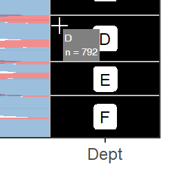
If the mouse cursor is not hovering over a stratum, we determine whether it is hovering over an alluvium polygon and if so, display different information in the tooltip.
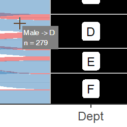
If the mouse cursor is hovering over an empty region of the plot, `renderText()` returns nothing and no tooltip appears.

Let's take a deeper dive into the logic used to determine the text that appears in the tooltip.
First, we check whether the cursor is inside the plot panel. If it is not, the element `plot_hover` of the input will be `NULL`. In that case `renderText()` will return nothing and no tooltip will appear.
```{r, eval = FALSE}
output$tooltip <- renderText(
if(!is.null(input$plot_hover)) { ... }
...
)
```
#### Hovering over a stratum
Next, we check whether the cursor is over a stratum. We round the x-coordinate of the mouse cursor in data units to the nearest integer, then determine whether the x-coordinate is within `node_width/2` of that integer. If so, the mouse cursor is horizontally within the box. Here the `if`-`else` statement includes behavior to display the tooltip for a stratum if true, and an alluvium if false.
```{r, eval = FALSE}
hover <- input$plot_hover
x_coord <- round(hover$x)
if(abs(hover$x - x_coord) < (node_width / 2)) { ... } else { ... }
```
If the condition is true, we need to find the index of the row of the input data that goes with the stratum the cursor is on. The data frame `pbuilt$data[[2]]` includes columns `x`, `ymin`, and `ymax` that define the x-coordinate of the center of the stratum, and the minimum and maximum y-coordinates of the stratum. We find the row index of that data frame where `x` is equal to the rounded x-coordinate of the cursor, and the y-coordinate of the cursor falls between `ymin` and `ymax`.
```{r, eval = FALSE}
node_row <-
pbuilt$data[[2]]$x == x_coord & hover$y > pbuilt$data[[2]]$ymin & hover$y < pbuilt$data[[2]]$ymax
```
To find the information to display in the tooltip, we get the name of the stratum as well as its width from the data in `pbuilt`.
```{r, eval = FALSE}
node_label <- pbuilt$data[[2]]$stratum[node_row]
node_n <- pbuilt$data[[2]]$count[node_row]
```
Finally, we render a tooltip using the `div` tag. We provide the text to display as arguments to `htmltools::renderTags()`. We also paste CSS style information together and pass it to the `style` argument. Note that the tooltip positioning is provided in CSS coordinates (pixels), not data coordinates. This does not require any additional effort on our part because `plot_hover` also includes an element called `coords_css`, which contains the mouse cursor location in pixel units.
```{r render strata tooltip, eval = FALSE}
renderTags(
tags$div(
node_label, tags$br(),
"n =", node_n,
style = paste0(
"position: absolute; ",
"top: ", hover$coords_css$y + offset, "px; ",
"left: ", hover$coords_css$x + offset, "px; ",
"background: gray; ",
"padding: 3px; ",
"color: white; "
)
)
)$html
```
#### Hovering over an alluvium
If the cursor is not over a stratum, the next nested `if`-statement checks whether it is over an alluvium. This is done using the function `sp::point.in.polygon()` applied across each of the polygons for which we defined the coordinates inside the `renderPlot()` expression.
```{r test within polygon, eval = FALSE}
hover_within_flow <- sapply(
polygon_coords,
function(pol) point.in.polygon(point.x = hover$x,
point.y = hover$y,
pol.x = pol$x,
pol.y = pol$y)
)
```
If at least one polygon is beneath the mouse cursor, we locate the corresponding row in the input data and extract information to display in the tooltip. (If the condition is not met, that means the cursor is hovering over an empty area of the plot, so no tooltip appears.)
```{r, eval = FALSE}
if (any(hover_within_flow)) { ... }
```
In the situation where there are more than one polygon overlapping, we get the information for the polygon that is plotted last by calling `rev()` on the logical vector returned by `point.in.polygon()`. This means that the tooltip will display information from the alluvium that appears "on top" in the plot. In this example, we display the names of the nodes that the alluvium connects, with arrows between them, and the width of the alluvium.
```{r info for alluvia tooltip, eval = FALSE}
coord_id <- rev(which(hover_within_flow == 1))[1]
flow_label <- paste(groups_to_draw[[coord_id]]$stratum, collapse = ' -> ')
flow_n <- groups_to_draw[[coord_id]]$count[1]
```
We render a tooltip using identical syntax to the one above.
```{r render alluvia tooltip, eval = FALSE}
renderTags(
tags$div(
flow_label, tags$br(),
"n =", flow_n,
style = paste0(
"position: absolute; ",
"top: ", hover$coords_css$y + offset, "px; ",
"left: ", hover$coords_css$x + offset, "px; ",
"background: gray; ",
"padding: 3px; ",
"color: white; "
)
)
)$html
```
## App with long-format alluvial data
The `vaccinations` dataset is used for long-format alluvial data. The app is embedded at the bottom of this document, but we don't need to walk through the source code because it's almost identical to the code above. The output of `ggplot_build()` that is used to find the polygon coordinates and information for the tooltips has a consistent structure regardless of the initial format of the input data. Therefore, the calculation of polygon coordinates, user interface, and server functions of the two apps are identical. The only difference is in the initial creation of the `ggplot()` object. Refer back to the [primary vignette](ggalluvial.html) for several example plots made both with long and with wide data.
The app is embedded below.
Again, if the app doesn't display in the window above for whatever reason, you can view it locally by running this line of code in your console:
```{r run long app locally, eval = FALSE}
shiny::shinyAppDir(system.file("examples/ex-shiny-long-data", package="ggalluvial"))
```
## Conclusion
This vignette demonstrates how to enable tooltips for {ggalluvial} plots in Shiny apps. This is one of many possible ways to do that. It may not be the optimal way — other solutions are certainly possible!
The full source code for both of these Shiny apps is included with the {ggalluvial} package in the 'examples' subdirectory where the package is installed: the source files are `ggalluvial/examples/ex-shiny-wide-data/app.R` and `ggalluvial/examples/ex-shiny-long-data/app.R`.
ggalluvial/vignettes/order-rectangles.rmd 0000644 0001762 0000144 00000053140 14370022542 020357 0 ustar ligges users ---
title: "The Order of the Rectangles"
author: "Jason Cory Brunson"
date: "`r Sys.Date()`"
output:
rmarkdown::html_vignette
vignette: >
%\VignetteIndexEntry{order of rectangles}
%\VignetteEngine{knitr::rmarkdown}
\usepackage[utf8]{inputenc}
---
How the strata and lodes at each axis are ordered, and how to control their order, is a complicated but essential part of {ggalluvial}'s functionality. This vignette explains the motivations behind the implementation and explores the functionality in greater detail than the examples.
## Setup
```{r setup}
knitr::opts_chunk$set(fig.width = 6, fig.height = 3, fig.align = "center")
library(ggalluvial)
```
All of the functionality discussed in this vignette is exported by {ggalluvial}. We'll also need a toy data set to play with. I conjured the data frame `toy` to be nearly as small as possible while complex enough to illustrate the positional controls:
```{r data}
# toy data set
set.seed(0)
toy <- data.frame(
subject = rep(LETTERS[1:5], times = 4),
collection = rep(1:4, each = 5),
category = rep(
sample(c("X", "Y"), 16, replace = TRUE),
rep(c(1, 2, 1, 1), times = 4)
),
class = c("one", "one", "one", "two", "two")
)
print(toy)
```
The subjects are classified into categories at each collection point but are also members of fixed classes.
Here's how {ggalluvial} visualizes these data under default settings:
```{r plot}
ggplot(toy, aes(x = collection, stratum = category, alluvium = subject)) +
geom_alluvium(aes(fill = class)) +
geom_stratum()
```
## Motivations
The amount of control the stat layers `stat_alluvial()` and `stat_flow()` exert over the [positional aesthetics](https://ggplot2.tidyverse.org/reference/aes_position.html) of graphical objects (grobs) is unusual, by the standards of {ggplot2} and many of its extensions. In [the layered grammar of graphics framework](https://www.tandfonline.com/doi/abs/10.1198/jcgs.2009.07098), the role of a statistical transformation is usually to summarize the original data, for example by binning (`stat_bin()`) or by calculating quantiles (`stat_qq()`). These transformed data are then sent to geom layers for positioning. The positions of grobs may be adjusted after the statistical transformation, for example when points are jittered (`geom_jitter()`), but the numerical data communicated by the plot are still the product of the stat.
In {ggalluvial}, the stat layers exert slightly more control.
For one thing, the transformation is more sophisticated than a single value or a fixed-length vector, such as a mean, standard deviation, or five-number summary. Instead, the values of `y` (which default to `1`) within each collection are, after reordering, transformed using `cumsum()` and some additional arithmetic to obtain coordinates for the centers `y` and lower and upper limits `ymin` and `ymax` of the strata representing the categories.
Additionally, the reordering of lodes within each collection relies on a hierarchy of sorting variables, based on the strata at nearby axes as well as the present one and, optionally, on the values of differentiation aesthetics like `fill`. How this hierarchy is invoked depends on the choices of several plotting parameters (`decreasing`, `reverse`, and `absolute`).
Thus, the results of the statistical transformations are not as intrinsically meaningful as others and are subject to much more intervention by the user.
Only once the transformations have produced these coordinates do the geom layers use them to position the rectangles and splines that constitute the plot.
There are two key reasons for this division of labor:
1. The coordinates returned by some stat layers can be coupled with multiple geom layers. For example, all four geoms can couple with the `alluvium` stat. Moreover, as showcased in [the examples](http://corybrunson.github.io/ggalluvial/reference/index.html), the stats can also meaningfully couple with exogenous geoms like `text`, `pointrange`, and `errorbar`. (In principle, the geoms could also couple with exogenous stats, but i haven't done this or seen it done in the wild.)
2. Different parameters control the calculations of the coordinates (e.g. `aes.bind` and `cement.alluvia`) and the rendering of the graphical elements (`width`, `knot.pos`, and `aes.flow`), and it makes intuitive sense to handle these separately. For example, the heights of the strata and lodes convey information about the underlying data, whereas their widths are arbitrary.
(If the data are provided in alluvia format, then `Stat*$setup_data()` converts them to lodes format in preparation for the main transformation. This can be done manually using [the exported conversion functions](http://corybrunson.github.io/ggalluvial/reference/alluvial-data.html), and this vignette will assume the data are already in lodes format.)
## Positioning strata
Each stat layer demarcates one stack for each data collection point and one rectangle within each stack for each (non-empty) category.[^yneg] In [{ggalluvial} terms](http://corybrunson.github.io/ggalluvial/articles/ggalluvial.html), the collection points are axes and the rectangles are strata or lodes.
[^yneg]: The one exception, discussed below, is for stratum variables that take both positive and negative values.
To generate a sequence of stacked bar plots with no connecting flows, only the aesthetics `x` (standard) and `stratum` (custom) are required:
```{r strata}
# collection point and category variables only
data <- structure(toy[, 2:3], names = c("x", "stratum"))
# required fields for stat transformations
data$y <- 1
data$PANEL <- 1
# stratum transformation
StatStratum$compute_panel(data)
```
Comparing this output to `toy`, notice first that the data have been aggregated: Each distinct combination of `x` and `stratum` occupies only one row.
`x` encodes the axes and is subject to layers specific to this positional aesthetic, e.g. `scale_x_*()` transformations.
`ymin` and `ymax` are the lower and upper bounds of the rectangles, and `y` is their vertical centers. Each stacked rectangle begins where the one below it ends, and their heights are the numbers of subjects (or the totals of their `y` values, if `y` is passed a numerical variable) that take the corresponding category value at the corresponding collection point.
Here's the plot this strata-only transformation yields:
```{r strata plot}
ggplot(toy, aes(x = collection, stratum = category)) +
stat_stratum() +
stat_stratum(geom = "text", aes(label = category))
```
In this vignette, i'll use the `stat_*()` functions to add layers, so that the parameters that control their behavior are accessible via tab-completion.
### Reversing the strata
Within each axis, `stratum` defaults to reverse order so that the bars proceed in the original order from top to bottom. This can be overridden by setting `reverse = FALSE` in `stat_stratum()`:
```{r strata reverse}
# stratum transformation with strata in original order
StatStratum$compute_panel(data, reverse = FALSE)
ggplot(toy, aes(x = collection, stratum = category)) +
stat_stratum(reverse = FALSE) +
stat_stratum(geom = "text", aes(label = category), reverse = FALSE)
```
**Warning:** The caveat to this is that, _if `reverse` is declared in any layer, then it must be declared in every layer_, lest the layers be misaligned.
This includes any `alluvium`, `flow`, and `lode` layers, since their graphical elements are organized within the bounds of the strata.
### Sorting the strata by size
When the strata are defined by a character or factor variable, they default to the order of the variable (lexicographic in the former case). This can be overridden by the `decreasing` parameter, which defaults to `NA` but can be set to `TRUE` or `FALSE` to arrange the strata in decreasing or increasing order in the `y` direction:
```{r strata decreasing}
# stratum transformation with strata in original order
StatStratum$compute_panel(data, reverse = FALSE)
ggplot(toy, aes(x = collection, stratum = category)) +
stat_stratum(decreasing = TRUE) +
stat_stratum(geom = "text", aes(label = category), decreasing = TRUE)
```
**Warning:** The same caveat applies to `decreasing` as to `reverse`: Make sure that all layers using alluvial stats are passed the same values!
Henceforth, we'll use the default (reverse and categorical) ordering of the strata themselves.
## Positioning lodes within strata
### Alluvia and flows
In the strata-only plot, each subject is represented once at each axis.
_Alluvia_ are x-splines that connect these multiple representations of the same subjects across the axes. In order to avoid having these splines overlap at the axes, the `alluvium` stat must stack the alluvial cohorts---subsets of subjects who have a common profile across all axes---within each stratum. These smaller cohort-specific rectangles are the _lodes_.
This calculation requires the additional custom `alluvium` aesthetic, which identifies common subjects across the axes:
```{r alluvia}
# collection point, category, and subject variables
data <- structure(toy[, 1:3], names = c("alluvium", "x", "stratum"))
# required fields for stat transformations
data$y <- 1
data$PANEL <- 1
# alluvium transformation
StatAlluvium$compute_panel(data)
```
The transformed data now contain _one row per cohort_---instead of per category---_per collection point_. The vertical positional aesthetics describe the lodes rather than the strata, and the `group` variable encodes the `alluvia` (a convenience for the geom layer, and the reason that {ggalluvial} stat layers ignore variables passed to `group`).
Here's how this transformation translates into the alluvial plot that began the vignette, labeling the subject of each alluvium at each intersection with a stratum:
```{r alluvia plot}
ggplot(toy, aes(x = collection, stratum = category, alluvium = subject)) +
stat_alluvium(aes(fill = class)) +
stat_stratum(alpha = .25) +
stat_alluvium(geom = "text", aes(label = subject))
```
The `flow` stat differs from the `alluvium` stat by allowing the orders of the lodes within strata to differ from one side of an axis to the other. Put differently, the `flow` stat allows _mixing_ at the axes, rather than requiring that each case or cohort is follows a continuous trajectory from one end of the plot to the other. As a result, flow plots are often much less cluttered, the trade-off being that cases or cohorts cannot be tracked through them.
```{r flows}
# flow transformation
StatFlow$compute_panel(data)
```
The `flow` stat transformation yields _one row per cohort per side per flow_. Each intermediate axis appears twice in the data, once for the incoming flow and once for the outgoing flow. (The starting and ending axes only have rows for outgoing and incoming flows, respectively.)
Here is the flow version of the preceding alluvial plot, labeling each side of each flow with the corresponding subject:
```{r flows plot}
ggplot(toy, aes(x = collection, stratum = category, alluvium = subject)) +
stat_stratum() +
stat_flow(aes(fill = class)) +
stat_flow(geom = "text",
aes(label = subject, hjust = after_stat(flow) == "to"))
```
The [computed variable](https://ggplot2.tidyverse.org/reference/aes_eval.html) `flow` indicates whether each row of the `compute_panel()` output corresponds to a flow _to_ or _from_ its axis; the values are used to nudge the labels toward their respective flows (to avoid overlap). Mismatches between adjacent labels indicate where lodes are ordered differently on either side of a stratum.
### Lode guidance
As the number of strata at each axis grows, heterogeneous cases or cohorts can produce highly complex alluvia and very messy plots. {ggalluvial} mitigates this by strategically arranging the lodes---the intersections of the alluvia with the strata---so as to reduce their crossings between adjacent axes.
This strategy is executed locally: At each axis (call it the _index_ axis), the order of the lodes is guided by several totally or partially ordered variables. In order of priority:
1. the strata at the index axis
2. the strata at the other axes to which the index axis is linked by alluvia or flows---namely, all other axes in the case of an alluvium, or a single adjacent axis in the case of a flow
3. the alluvia themselves, i.e. the variable passed to `alluvium`
In the alluvium case, the prioritization of the remaining axes is determined by a _lode guidance function_.
A lode guidance function can be passed to the `lode.guidance` parameter, which defaults to `"zigzag"`. This function puts the nearest (adjacent) axes first, then zigzags outward from there, initially (the "zig") in the direction of the closer extreme:
```{r lode zigzag}
for (i in 1:4) print(lode_zigzag(4, i))
```
Several alternative `lode_*()` functions are available:
- `"zagzig"` behaves like `"zigzag"` except initially "zags" toward the farther extreme.
- `"frontback"` and `"backfront"` behave like `"zigzag"` but extend completely in one outward direction from the index axis before the other.
- `"forward"` and `"backward"` put the remaining axes in increasing and decreasing order, regardless of the relative position of the index axis.
Two alternatives are illustrated below:
```{r alluvia plot w/ backfront guidance}
for (i in 1:4) print(lode_backfront(4, i))
ggplot(toy, aes(x = collection, stratum = category, alluvium = subject)) +
stat_alluvium(aes(fill = class), lode.guidance = "backfront") +
stat_stratum() +
stat_alluvium(geom = "text", aes(label = subject),
lode.guidance = "backfront")
```
The difference between `"backfront"` guidance and `"zigzag"` guidance can be seen in the order of the lodes of the `"Y"` stratum at axis `3`: Whereas `"zigzag"` minimized the crossings between axes `3` and `4`, locating the distinctive class-`"one"` case above the others, `"backfront"` minimized the crossings between axes `2` and `3` (axis `2` being immediately before axis `3`), locating this case below the others.
```{r alluvia plot w/ backward guidance}
for (i in 1:4) print(lode_backward(4, i))
ggplot(toy, aes(x = collection, stratum = category, alluvium = subject)) +
stat_alluvium(aes(fill = class), lode.guidance = "backward") +
stat_stratum() +
stat_alluvium(geom = "text", aes(label = subject),
lode.guidance = "backward")
```
The effect of `"backward"` guidance is to keep the right part of the plot as tidy as possible while allowing the left part to become as messy as necessary. (`"forward"` has the opposite effect.)
### Aesthetic binding
It often makes sense to bundle together the cases and cohorts that fall into common groups used to assign differentiation aesthetics: most commonly `fill`, but also `alpha`, which controls the opacity of the `fill` colors, and `colour`, `linetype`, and `size`, which control the borders of the alluvia, flows, and lodes.
The `aes.bind` parameter defaults to `"none"`, in which case aesthetics play no role in the order of the lodes. Setting the parameter to `"flows"` prioritizes any such aesthetics _after_ the strata of any other axes but _before_ the alluvia of the index axis (effectively ordering the flows at each axis by aesthetic), while setting it to `"alluvia"` prioritizes aesthetics _before_ the strata of any other axes (effectively ordering the alluvia).
In the toy example, the stronger option results in the lodes within each stratum being sorted first by class:
```{r alluvia plot w/ strong aesthetic binding}
ggplot(toy, aes(x = collection, stratum = category, alluvium = subject)) +
stat_alluvium(aes(fill = class, label = subject), aes.bind = "alluvia") +
stat_stratum() +
stat_alluvium(geom = "text", aes(fill = class, label = subject),
aes.bind = "alluvia")
```
The more flexible option groups the lodes by class only after they've been ordered according to the strata at the remaining axes:
```{r alluvia plot w/ weak aesthetic binding}
ggplot(toy, aes(x = collection, stratum = category, alluvium = subject)) +
stat_alluvium(aes(fill = class, label = subject), aes.bind = "flows") +
stat_stratum() +
stat_alluvium(geom = "text", aes(fill = class, label = subject),
aes.bind = "flows")
```
**Warning:** In addition to parameters like `reverse`, _when aesthetic variables are prioritized at all, overlaid alluvial layers must include the same aesthetics in the same order_. (This can produce warnings when the aesthetics are not recognized by the geom.) Try removing `fill = class` from the text geom above to see the risk posed by neglecting this check.
Rather than ordering lodes _within_, the `flow` stat separately orders the flows _into_ and _out from_, each stratum. (This precludes a corresponding `"alluvia"` option for `aes.bind`.)
By default, the flows are ordered with respect first to the orders of the strata at the present axis and second to those at the adjacent axis.
Setting `aes.bind` to the non-default option `"flows"` tells `stat_flow()` to prioritize flow aesthetics after the strata of the index axis but before the strata of the adjacent axis:
```{r flows plots w/ aesthetic binding}
ggplot(toy, aes(x = collection, stratum = category, alluvium = subject)) +
stat_flow(aes(fill = class, label = subject), aes.bind = "flows") +
stat_stratum() +
stat_flow(geom = "text",
aes(fill = class, label = subject,
hjust = after_stat(flow) == "to"),
aes.bind = "flows")
```
Note: The `aes.flow` parameter tells `geom_flow()` how flows should inherit differentiation aesthetics from adjacent axes---`"forward"` or `"backward"`. It does _not_ influence their positions.
### Manual lode ordering
Finally, one may wish to put the lodes at each axis in a predefined order, subject to their being located in the correct strata. This can be done by passing a data column to the `order` aesthetic.
For the toy example, we can pass a vector that puts the cases in the order of their IDs in the data at every axis:
```{r alluvia plot w/ manual lode ordering}
lode_ord <- rep(seq(5), times = 4)
ggplot(toy, aes(x = collection, stratum = category, alluvium = subject)) +
stat_alluvium(aes(fill = class, order = lode_ord)) +
stat_stratum() +
stat_alluvium(geom = "text",
aes(fill = class, order = lode_ord, label = subject))
```
```{r flows plot w/ manual lode ordering}
ggplot(toy, aes(x = collection, stratum = category, alluvium = subject)) +
stat_flow(aes(fill = class, order = lode_ord)) +
stat_stratum() +
stat_flow(geom = "text",
aes(fill = class, order = lode_ord, label = subject,
hjust = after_stat(flow) == "to"))
```
Within each stratum at each axis, the cases are now in order from top to bottom.
## Negative strata
In response to an elegant real-world use case, {ggalluvial} can now handle negative observations in the same way as `geom_bar()`: by grouping these observations into negative strata and stacking these strata in the negative `y` direction (i.e. in the opposite direction of the positive strata). This new functionality complicates the above discussion in two ways:
1. _Positioning strata:_ The negative strata could be reverse-ordered with respect to the positive strata, as in `geom_bar()`, or ordered in the same way (vertically, without regard for sign).
2. _Positioning lodes within strata:_ Two strata may correspond to the same stratum variable at an axis (one positive and one negative), which under-determines the ordering of lodes within strata.
The first issue is binary: Once `decreasing` and `reverse` are chosen, there are only two options for the negative strata. The choice is made by setting the new `absolute` parameter to either `TRUE` (the default), which yields a mirror-image ordering, or `FALSE`, which adopts the same vertical ordering.
This setting also influences the ordering of lodes within strata at the same nexus as `reverse`, namely at the level of the alluvium variable.
The second issue is then handled by creating a `deposit` variable with unique values corresponding to each _signed_ stratum variable value, in the order prescribed by `decreasing`, `reverse`, and `absolute`. The `deposit` variable is then used in place of `stratum` for all of the lode-ordering tasks above.
As a point of reference, here is a bar plot of the toy data, with a randomized sign variable used to indicate negative-valued observations:
```{r bar plot with negative observations}
set.seed(78)
toy$sign <- sample(c(-1, 1), nrow(toy), replace = TRUE)
print(toy)
ggplot(toy, aes(x = collection, y = sign)) +
geom_bar(aes(fill = class), stat = "identity")
```
The default behavior, illustrated here with flows, is for the positive strata to proceed downward and the negative strata to proceed upward, in both cases from larger absolute values to zero:
```{r flows plot w/ negative strata}
ggplot(toy, aes(x = collection, stratum = category, alluvium = subject,
y = sign)) +
geom_flow(aes(fill = class)) +
geom_stratum() +
geom_text(stat = "stratum", aes(label = category))
```
To instead have the strata proceed downward at each axis, and the lodes downward within each stratum, set `absolute = FALSE` (now plotting alluvia):
```{r alluvia plot w/ negative strata}
ggplot(toy, aes(x = collection, stratum = category, alluvium = subject,
y = sign)) +
geom_alluvium(aes(fill = class), absolute = FALSE) +
geom_stratum(absolute = FALSE) +
geom_text(stat = "alluvium", aes(label = subject), absolute = FALSE)
```
Note again that the labels are consistent with the alluvia and flows, despite the omission of the `fill` aesthetic from the text geom, because the aesthetic variables are not prioritized in the ordering of the lodes.
## More examples
More examples of all of the functionality showcased here can be found in the documentation for the `stat_*()` functions, [browsable on the package website](http://corybrunson.github.io/ggalluvial/reference/index.html).
## Appendix
```{r session info}
sessioninfo::session_info()
```
ggalluvial/vignettes/img/ 0000755 0001762 0000144 00000000000 14166562215 015175 5 ustar ligges users ggalluvial/vignettes/img/hover_empty_area.png 0000644 0001762 0000144 00000043216 14166562215 021242 0 ustar ligges users PNG
IHDR j 'SzTXtRaw profile type exif xڭi7s`?C)&U B{O\^O5?w|.K~>?./Ͽ}(iDׅׅR"|]`|f?NaN_Wכl.'xRH1 ?dѧ~k u??xyϋY~[;X~η=ٍ\Y5oSy?ɒ__g{;#{!~zvb'"zWe
7ZiM%w7ށwłR_^^|}_+CWE@G-Q\,o~~.1K-QzNSkX"]LHDאJ[؈BzRf1T N7Kfj2B V`#,7rhTr)+2jZU߰dيU3kmr+6k͵F=nঃ+>=x34,Nm9*.[ͭƎ;mpbm T:SvT[nvw|ZpߏZ"7Qo7Eo!:HU("F =vDos
"rN9n,܋PwmZ@nU]lNa{Jڭxn[
#O,7*jt(5a:k薊mb,yrhF/;:i>4]*Wf3VH)XQbc(mJ8;B[R'Xs5UM͏:z轄<R=P3kh%K]>:XlUeC+9]biq9ۓ59:sɪɗ;ST`^yj)
Aed7kxcgI=mF^==InX ; |/.כˈ;vbQEۨj͓rv:ZgF2f#
yoVTQme=E^dc3iw2ڛ l'b7ykhaȐc{;"s7ruE[ٖsa!nYjP*mo0;F) greT]uRn=\?nb9<Ʉ%ύtpzlr-)Jr4jQ8;DS ^`#ҩ@$TFuj:|J$GkQ6K' mߨNw;(jwvW@ڀ bfku!(uibnxg}p@`'^u@2nةodIy=wvn|=42yY3r5x7ejղ9@8|6Ȟ*,%H~7`I>kkŸ)EnFWCfNe @>^XeZh'VU|JrZCD:f#PV>/Rp~i=1
^_팜.ѡ